Adams has prescribed the Zones. 11 of them. This had consequences. In the digital case, it seems, severe ones.

To access all 11 zones on a sensor, the middle tone needs to be placed very low, 5 steps lower than sensor saturation, instead of 2.5 steps for 18% or 3 steps for 12.5%. 5 steps coincide with 3% (100/2^5 = 100/32).

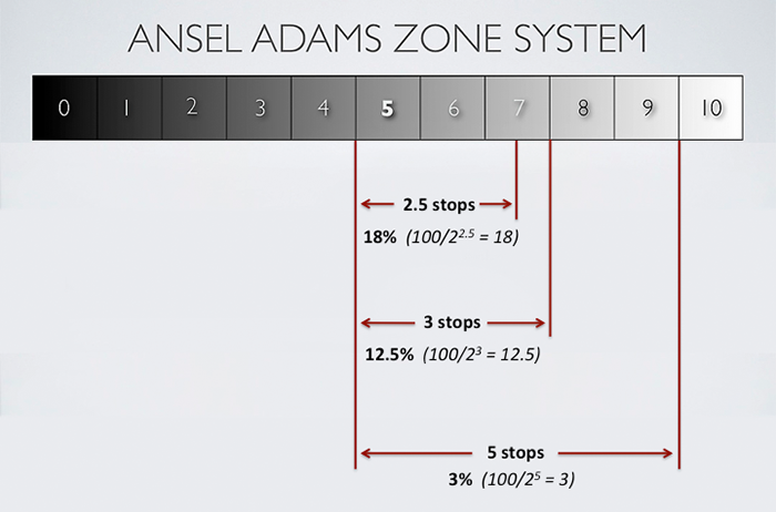
Figure 1.

Here goes a little bit, (really, just a bit) of mathematics. We're going to use a few simple mathematic formulae, which reflect the relationship between the amount of the change in EV units (photographic stops) and the change in linear counts (linear RAW values). Change in EV units is equal to log₂(the ratio of the second count to first count). Therefore, a 1 stop (+1 EV) change in exposure is equal to the 2x change (2^1) in linear raw count, like going from the count of 1000 to the count of 2000 if it is +1 EV; or going from the count of 1000 to the count of 500 if it is -1 EV. A change of 2 stops means changing the linear count 4 times, 1000 to 250 is -2 EV; 1000 to 4000 is +2EV. So, analogously, changing the exposure by 1/3 EV would be the same thing as changing the linear count by the cube root of 2, that is 1.26 times (1000 to 1260 for +1/3 EV), while changing the exposure by 1/2 EV is the same as changing the linear count by the square root of 2, 1.414 times (1000 to 1414 for +1/2 EV).

So, if we know the EV value, we can find by how much the linear count has changed by raising 2 to the power equal to the amount of change in EV units.

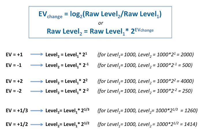
Figure 2.

Let's take the recent Olympus camera, OM-D E-M10. It records 12-bit RAW data with the maximum raw level reaching 3840, as we can see from the shot taken from Imaging Resource site and opened in RawDigger:

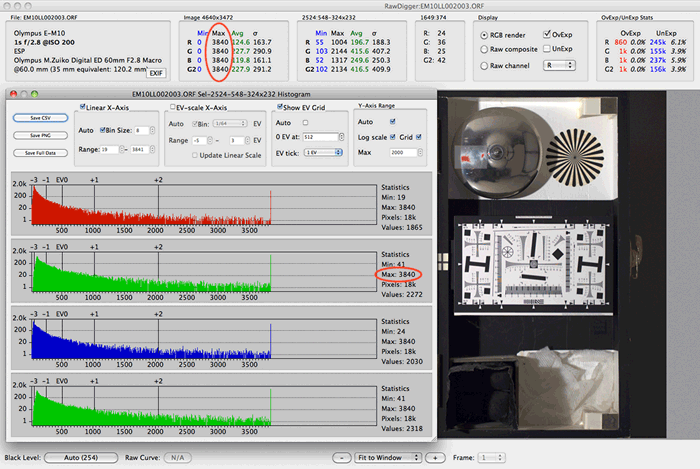
Figure 3.

Distributing those 3840 tones between all the zones and accounting for the while balance for the daylight, we get a fairly unpleasant situation - there are very few counts in the middle tone (zone V), while in the shadows, where we want details (zone II), they are practically non-existent. Total level count in the zone II is only 24 gradations (#R + 2*#G + #B = 4 + 2*8 + 4, where #G, number of levels in green channel, is multiplied by two because of the Bayer sensor arrangement, RGBG).

The reduced number of tones (or, in other words, limited number of levels per stop or zone) turns into the loss of detail resolution. Pulling details and color from those underexposed middle tones and shadows is very painful. Noise starts to raise its head, color smudges and blotches appear, the details become rough, and the image loses plasticity.

For instance, here is what the image looks like when shot with the settings that the camera suggests. As you can see, over 8% of pixels in the blue channel are underexposed.

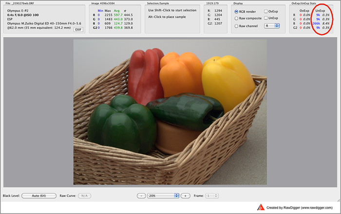
Figure 4.

For comparison, here is what an image statistics looks like when shot with, at least what the camera believes to be, 1 full stop of overexposure – as you can see, there is absolutely no overexposure, while the underexposure goes down significantly, 4+ times in pixel count.

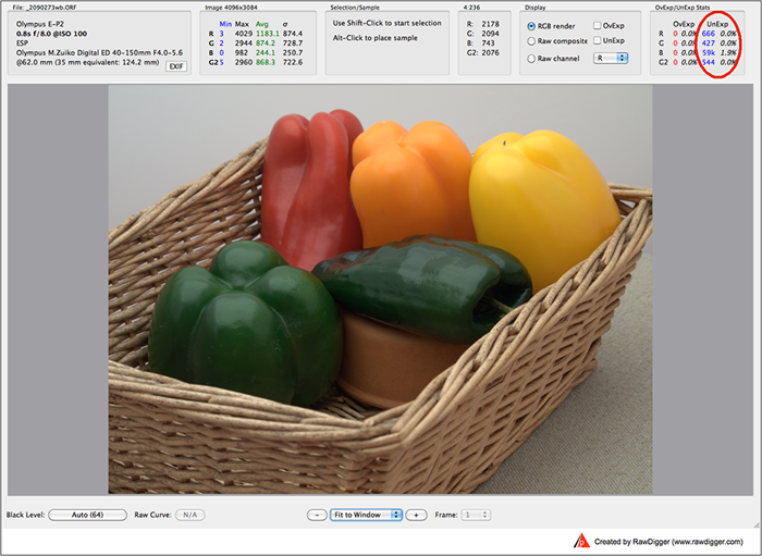
Figure 5.

Now, when processed with PhotoShop, this is how the ‘’overexposed’’ image shadows look:

Figure 6.

…and HERE are the same shadows on the image that was exposed according to the suggested camera.

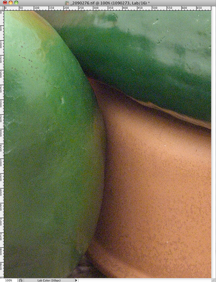
Figure 7.

As you can see, the noise is painfully obvious.

Other problems that you could encounter are color smudges and blotches, rough details, and loss of plasticity in the image.

Here is this underexposure in practice. The following shot is also by Imaging Resource, taken with the same Olympus OM-D E-M10 camera, set to the base ISO of 200:

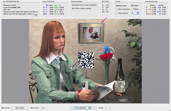
Figure 8.

In the overexposure and underexposure section (OvExp/UnExp Stats), it's visible that only 367+290 pixels in the green channels are blown out (saturated). These pixels are located on a few tiny specular highlights caused by curvatures on metallic surfaces such as the button on the jacket pocket and metal picture frame. Switching on the OvExp warning checkbox puts a red/purple overlay on saturated pixels. Turning the overexposure warning on and off one can see that there are also a few saturated pixels on the metal watch bracelet. For illustration purposes we also added three arrows pointing to those blown out highlights.

Such a small total amount of saturated pixels means that the image is in fact underexposed - with normal exposure, the specular highlights on metal and glass surfaces should indeed appear as specular highlights, not monotone featureless areas, which only lower the apparent contrast of the image and do not bring any artistic merit. However, +0.3 EV has already been manually added to the automatic exposure - this is visible in EXIF.

Let's press the EXIF button and see:

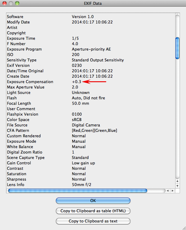
Figure 9.

How much does it make sense to further increase the exposure, and how will the overexposed areas change from said increase?

To control the overexposure warning, we’ve added a special feature to version 1.03 of RawDigger, see RawDigger Preferences -> Over/Under Exposure -> Overexposure Detection -> Auto OE Offset.

For instance, for the given image, let's simulate an additional exposure compensation of +1/2 stop during the shot, to do so let’s set a negative shift in the Auto OE Offset field:

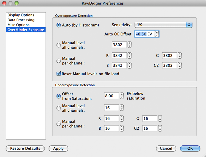
Figure 10.

Applying it, we see the following:

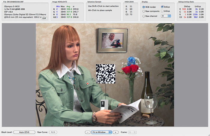
Figure 11.

Now, this is better. It seems that the camera calculated the exposure to be off by -0.8 EV (the manual exposure correction during the shoot for +0.3 EV, and + 0.5 EV, which we got evaluating the image in RawDigger).

OK. Let's consider the possibility that for the given scene the exposure automation was unable to "comprehend" that the dynamic range of the scene was increased due to the useless specular highlights, decided that they were important to keep from blowing out, and set the exposure to avoid losing them at the cost of lowering the overall exposure and thus causing more problems in shadows. But what if there were no metal or specular highlights?

Here's a shot with only auto exposure, without any manual correction at all, borrowed from Olympus OM-D E-M10 review by Quesabesde:

Figure 12.

The maximum turned out to be 2133, instead of the physically possible 3840, which is already, by itself, a sign of total underexposure by log₂(3840/2133)= 0.8 EV (see math above). The statistics for the underexposure are also quite unpleasant: 7% of pixels from the blue channels are in the underexposure zone (by default, RawDigger settings are set to a dynamic range of 8 stops; any lower, and, especially with 12-bit RAW, there are too few levels and the noise is too apparent – pulling out any useful color or details from below those 8 stops down from saturation is being too optimistic). To get an idea of what the underexposed areas are you can set the checkmark in UnExp checkbox, the areas marked with blue overlay are those underexposed.

Let's take a look at the RAW data histogram for this image (Window -> Histogram). To better see how the extreme highlights are recorded in the RAW, let's turn on the log scale for the Y-axis: over the histogram, in the "Y-Axis Range" section let's check the "Log Scale" checkbox. Next, in the "Show EV Grid" section, let's uncheck the "Auto" checkbox, and in the "0 EV at:" field let's input the real maximum of 3840: now the step countdown starts from this maximum value and goes into the negative, with helps to determine the amount of stops the image is underexposed by.

The histogram with the controls set as per above looks like this:

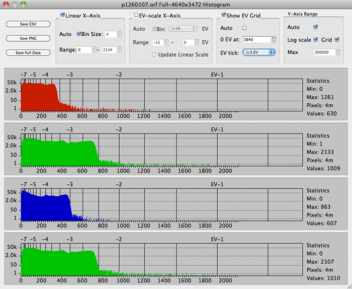
Figure 13.

On the vertical axis we see the number of pixels that were recorded in RAW to have certain level. The value of the level is shown on the lower horizontal axis. The upper horizontal axis of the histogram has a logarithmic log₂ scale,and is divided by stops of exposure, where a step is controlled in the same section "Show EV Grid", in the "EV Tick" field.

The part of the histogram in the highlight area (the right part, high level values), where the bulk of the levels are occurring 1-2 times, can be cut off without losing any information important to the scene, by just increasing the exposure during the shoot (to have a clear view of those levels which occur only 1 or 2 times creating ringing in the highlights we set Y-axis to logarithmic scale, because if the logarithmic scale is switched off that chatter is going below radar).

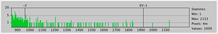
Figure 14.

The "ones" in the green channel end at about -2 EV, which means that the shot is underexposed by at least 2 stops, which corresponds to a 4^х- scale decrease in the RAW levels of the scene itself. In other words, the 12-bit camera becomes a 10-bit.

Let’s set the "Auto OE Offset" field to -2 EV, imitating in this manner a +2 EV exposure compensation during the shoot:

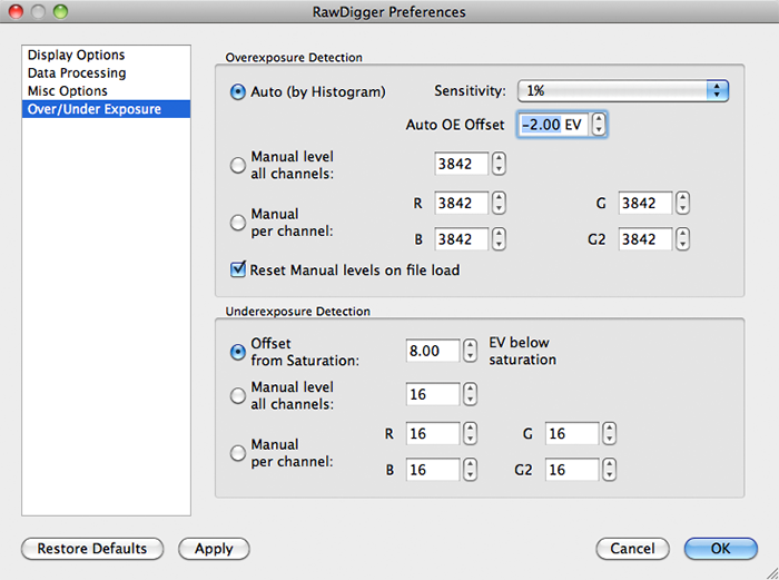
Figure 15.

Statistics show that only a few pixels were "overexposed", while the number of pixels in the underexposed zone decreased to a negligibly small amount and essentially the underexposure is now gone:

Figure 16.

Realistically, we could add another 1/3 of a stop. Doing so, we will get a few tiny specular highlights on the bends and edges of the candy wrappers. Let's put -2.3 in the "Auto OE Offset" field, and get just a little over 800 "overexposed" pixels in total in all of the channels:

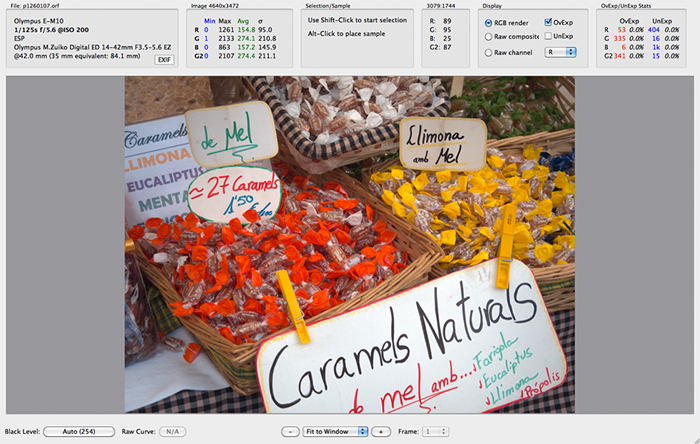
Figure 17.

It turns out that the auto exposure regardless of the dynamic range of the scene tends to decrease the exposure by two stops, leaving space “just in case” even for the shots where such decrease is not required. No camera intellect seems to affect this decision-making. For high-contrast scenes with really important details in highlights this somehow works, while for relatively low-contrast the underexposure is from something like 2/3 to really dramatic 2 1/3 stops.

Let’s have a look at the underexposed areas – that is, deep shadows below 8 stops under the saturation, for the “uncorrected” image and for the image where we simulated +2.3 EV exposure compensation. Switching on the UnExp warning we see those pixels below -8 EV from saturation covered with blue overlay. For the uncorrected image the underexposed areas are very significant.

Figure 18.

For the image where we simulated the hotter exposure the underexposed areas are pretty much absent.

Figure 19.

One of the most important challenges for a camera manufacturer is to produce a good-looking JPEG in the camera and to avoid blowing highlights as much as possible. To meet this challenge many cameras by default are programmed to underexpose. Underexposure is caused by the attempt of the camera manufacturer to cover all zones by overstating the ISO values and calibrating the camera meter accordingly. One can’t notice this while evaluating the exposure by looking at the brightness of out-of-camera JPEGs (OOC JPEGs) as the underexposure is counteracted by quite a strong midtone-brightening tone curve, which is applied before the JPEG and camera histogram are calculated.

For example, here you can see the embedded JPEG for the original underexposed shot:

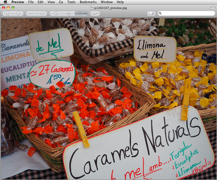
Figure 20. JPEG as shot

Same, most raw converters apply a similar curve by default as soon as a RAW file is opened making it harder to see what the real exposure-in-the-RAW is. In effect, we have a rather rigid system consisting of exposure meter calibration, sensor calibration, and tone curve optimized to produce most good-looking OOC JPEGs.

Bending this system by applying exposure compensation becomes difficult due to skewed feedback on the camera LCD (if only one is using it to evaluate exposure).

Suppose we would expose the caramels hotter by 2.3 EV and here is about what we will see on the camera LCD (simulated via Adobe Camera Raw):

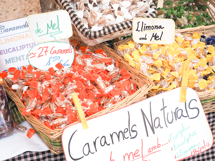
Figure 21. Embedded JPEG brightened by 2.3 EV

It is too bright now, details and colors are washed out and the scene looks overexposed by at least two stops.

Below you can see overexposure warning in ACR. It is approximately how the in-camera LCD would indicate it, too. From this overexposure indication it seems the shot is ruined, while in fact it is perfectly OK:

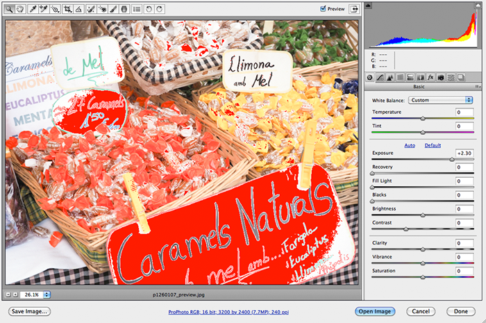
Figure 22.

When the tone curve pushes the midtones it also compresses the highlights causing them to lose details and texture when viewed on the camera LCD. As with slide film, this sometimes results in the desire to underexpose even more, say, to get some texture in the clouds. More often than not, the necessary details are already there in RAW, but camera preview tricks to believe highlights are void. Total underexposure mounts while most cameras do not offer any good tools to visualize underexposure, as if all we are concerned with is keeping highlights from being blown out.

If we take the OOC JPEG as displayed on the back of the camera as a good approximation of the look of the finished photo we need to expose for the tone curve, just as it is with film E-6 process – if, of course, one wants an immediately usable transparency without any re-touching, scanning, duplicating, or other additional processing.

To the contrary, exposing for the dynamic range of the scene demands photographer’s intervention, often on the shot-by-shot basis, during the raw conversion. This is not how automatic in-camera JPEG engines operate. In a sense OOC JPEG is an enemy of a RAW shooter, since having usable OOC JPEGs + keeping highlights through underexposure strategy places unnecessary restrictions on the camera’s exposure system.

Figure 23. As shot

… and now with underexposed area highlighted:

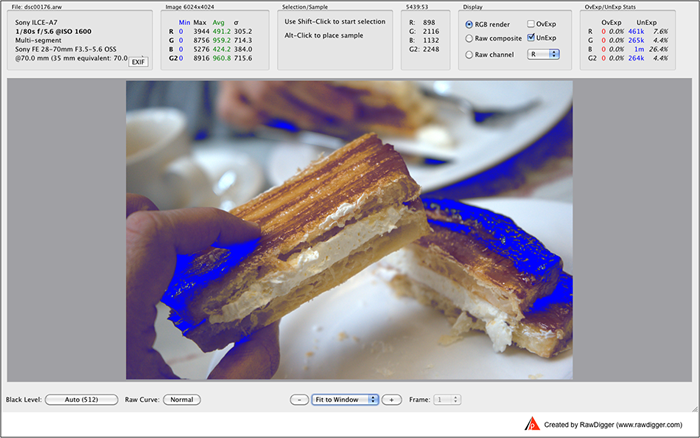
Figure 24.

If it would have been exposed hotter by 3.0 EV:

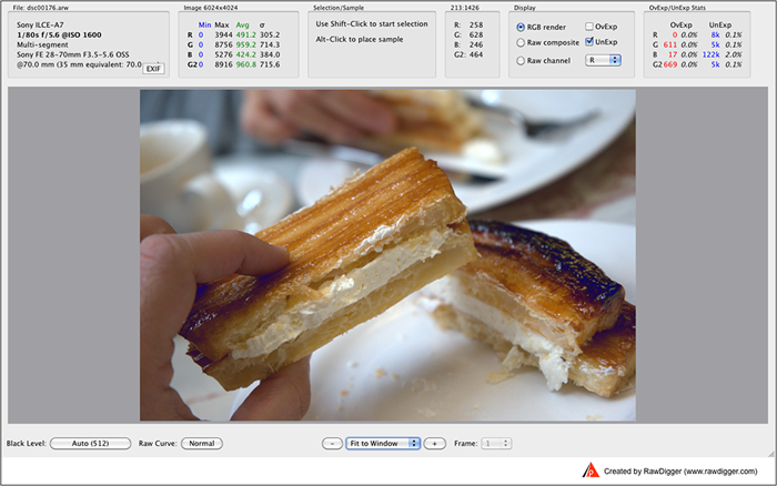
Figure 25.

The exposure parameters were already at the limits (high ISO, slow shutter, fully opened aperture), so a diffused flash might be a good idea. In a studio one can additionally use a tilt lens.

It seems now, that everything new - is just forgotten old, and a photographer needs to set the exposure compensation after evaluating the scene, sometimes with a spotmeter, considering the contrast of the scene between the details in the shadows and the details in the highlights he wishes to keep; and to use bracketing.

It is also good to remember that not every scene can be turned into a good shot by using proper camera settings even when combined with post-processing. Let’s look at this shot:

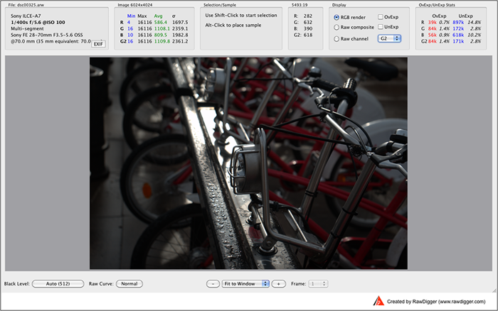
Figure 26.

… and now with overexposed and underexposed areas highlighted:

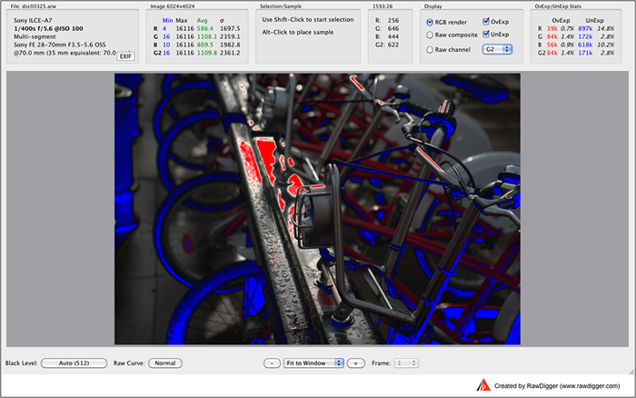
Figure 27. As shot displaying over- and underexposed areas

Sometimes it is better just to shoot from a different angle, wait for better light, use fill light, apply dulling spray or fine powder, etc. On this particular shot shadows could have been substantially better with a slower shutter speed, not causing much propagation of the blown-out area. But of course the question is – do we want that blown-out area in the center of the composition?

Of course, it's useful to tune the cameras settings (contrast, saturation, sharpening, color space, scene mode,…) so that the indicators for overexposure become more accurate, at least for close to neutral tones, and correspond to saturation values in RAW. However it is a difficult battle, accurate metering and bracketing seems to be both easier and more in the line with photographic practice.

The Unique Essential Workflow Tool

for Every RAW Shooter

FastRawViewer is a must have; it's all you need for extremely fast and reliable culling, direct presentation, as well as for speeding up of the conversion stage of any amounts of any RAW images of every format.

Now with Grid Mode View, Select/Deselect and Multiple Files operations, Screen Sharpening, Highlight Inspection and more.