
Submitted by Iliah Borg on
First published on PhotographyLife
"What happens to my mid-tones? I set exposure using exposure meter; open the shot in Adobe Lr (or Adobe Camera Raw, or some other converter) - the shot looks overexposed and everything starting from mid-tone and up looks very flat. If I shoot RAW+JPEG, JPEG looks OK, while RAW is not. Should I expose lower?"
Short Version
Please don't lower the exposure, you will be underexposing by more than 1 stop additionally to the underexposure due to camera meter calibration. Not a great idea, especially if the light is low and you are already above ISO 400.
As a result of lowering the exposure you will push shadows higher on the tone scale while doing raw conversion, thus transposing shadow noise and artifacts (such as banding and blotches) to lighter tones where they are more visible; consequently you will reduce resolution in those areas, as more noise and less levels in raw mean less details.
Instead, change the default settings in your raw converter (read on for a suggestion) or adjust on a per image basis. Having customized defaults, however, will save you a lot of time down the road.
While reading, please keep in mind that one can't judge the exposure by the brightness. Brightness is the product of the raw conversion process and as such depends on the settings in the raw converter, including the default settings, which may not be so obvious. Of course, brightness also depends on the monitor calibration and viewing conditions, as well as the ISO setting in the camera, much the same way the volume control sets the loudness. That, however, is a subject for another day.
First, let's see how this brightening happens in raw conversion.
Comparing RAW Rendered "As Is" to its Default Render in a Converter
Consider the following example.
When opening this shot in ACR or Adobe Lr (and in some other converters, too) it does look overexposed and flat on the higher tones (see the upper left part of the banana, it starts to lose volume, to look flat, glossy, nearly featureless; while persimmon is obviously too bright)
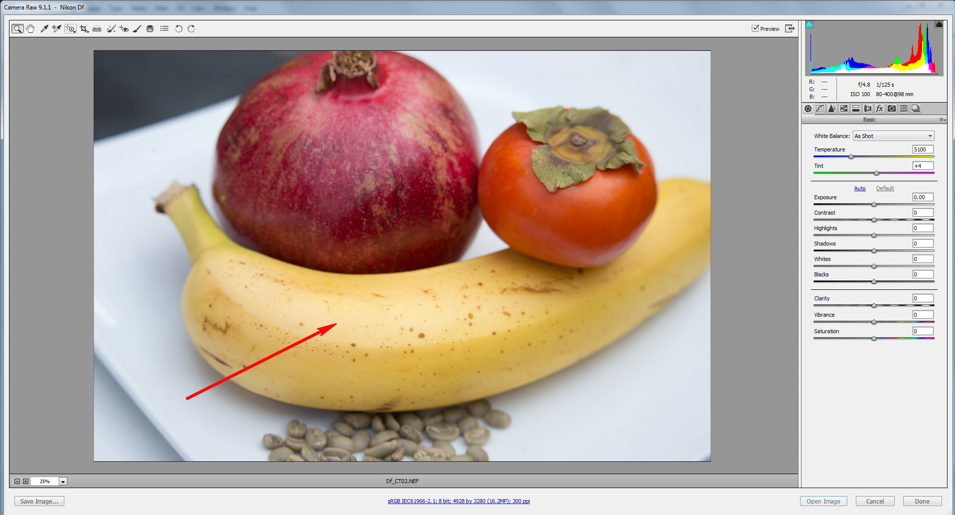
Figure 1. Df_CT02.NEF in ACR
Comparing it to the JPEG the camera recorded, the JPEG looks much less flat in that area (ironically, this is because my cameras are set to custom "flat" picture control, preventing extreme image brightening)
We can look at this embedded JPEG using FastRawViewer. This looks a little better.
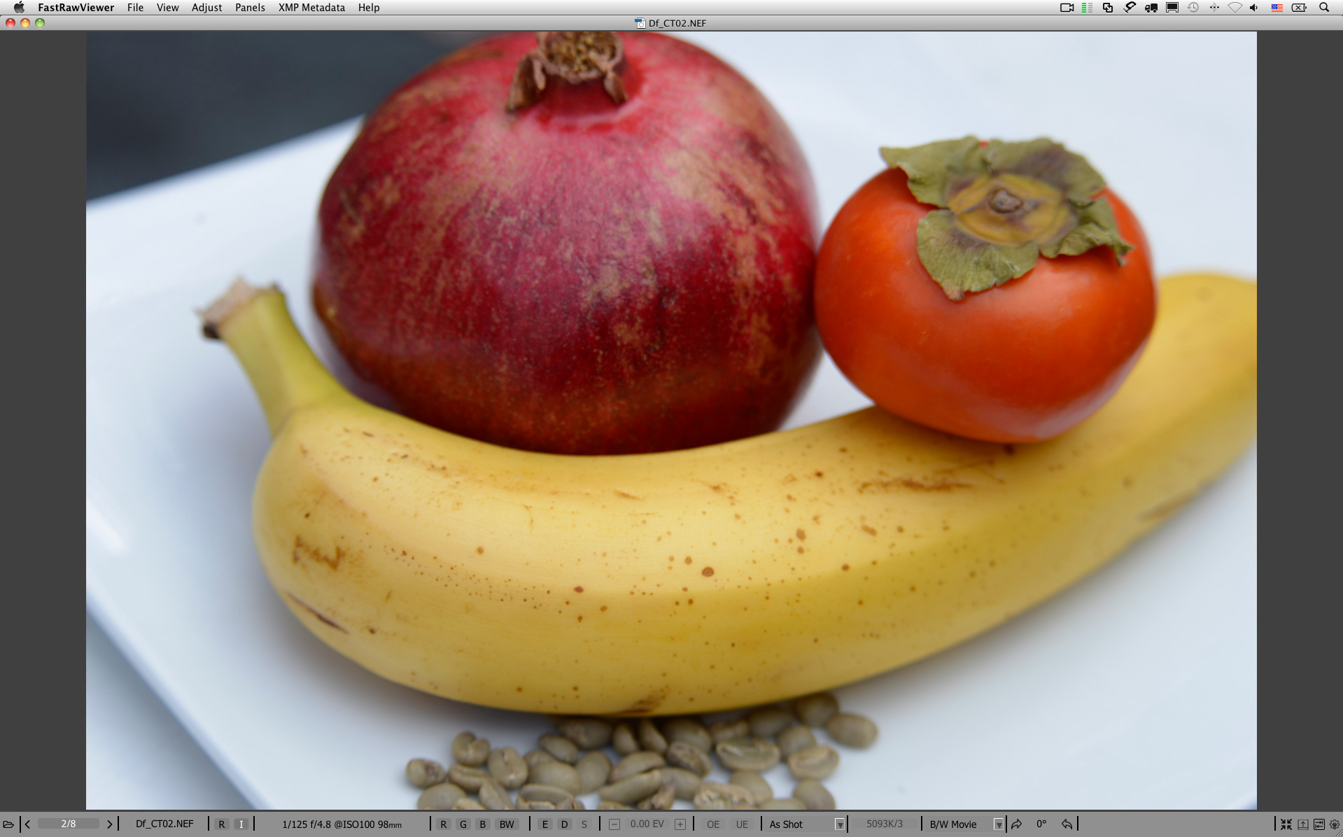
Figure 2. Df_CT02.NEF. Embedded JPEG in FastRawViewer
To see the raw truth, we can open the same raw shot in RawDigger, rendered "as is" without any adjustments applied:
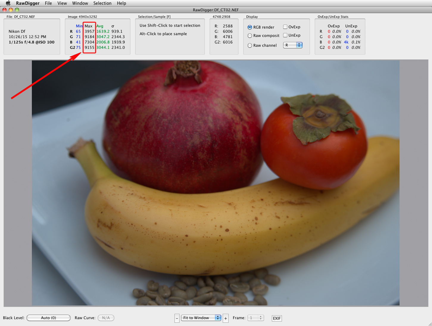
Figure 3. Df_CT02.NEF in RawDigger
- The previously marked (Figure 1) area of the shot does not look like it's been flattened into a pancake anymore
- The raw statistics and raw histogram indicate that not only is this shot NOT overexposed, as a matter of fact it is underexposed by nearly a stop (maximum is below 9200 on a 14-bit scale).
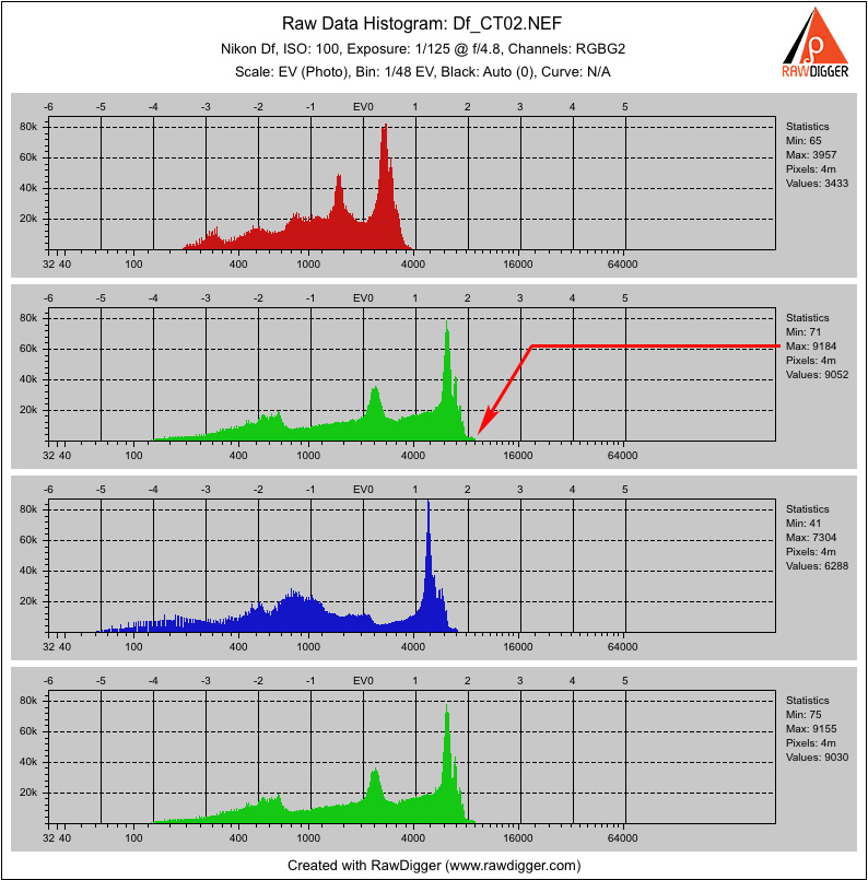
Figure 4. Df_CT02.NEF – raw histogram
So if you were to try and expose your shots to look good and properly exposed in a raw converter "as is", by default, you would need to underexpose this shot even more, close to 2 EV total.
It seems as if ACR (Figure 1) applies some default adjustments to a raw shot upon opening it.
Below we will calculate the exact value of the adjustment, applied by default to the midtone. If you are not into formulas and calculations you can scroll down to the next part, devoted to the practical advice on how to deal with those default adjustments.
Calculating the Brightening Caused by The Default Adjustments
Now we need something better than just a visual reference, as we are going to deal with numbers; and we need a shot of a target with known values.
The famous Kodak Q13 grey step wedge has known and stable values. It was designed to "find the correct exposure and processing conditions" and suits here very well. Q13 was sharing the first place among the most photographed objects in the world with Macbeth ColorChecker.
Figure 5. Kodak Q13 grey step wedge
From the Kodak formulation, the absolute reflection density Dr (we will shorten it to just "density" - D) of "A" patch is 0.05D, the step between patches is 0.1D. According to the formulation, the "M" patch receives the density of 0.75D (0.05 + 7*0.1D).
Following “A Guide to Understanding Graphic Arts Densitometry" by X-Rite, p.5:
| D = log10(1/Rf ), that is Rf = 1 /10^D, | (1) |
| where Rf is Reflectance factor (say, 0.18 for 18%) |
More details can be found in ISO 5-4:2009, but the above is sufficient for the task at hand.
Q13 is designed in such a way that the reflectance of the "M" patch in percentage (clipping point is considered to be 100% reflectance) is very close to the proverbial 18% mid-tone:
| 100% / (10^0.75) = 17.78% |
That is fortunate, as ISO Standard 12232 "Digital still cameras -- Determination of exposure index, ISO speed ratings, standard output sensitivity, and recommended exposure index" defines the midpoint on a rendered image as 18% grey.
To connect the dots, let's also see how to convert density D to familiar photographic stops, that is to EV units.
Given that for linear data:
| EV = log2(1/Rf) | (2) |
Hence, using formula (1), we will infer that the correlation between the density and EV units is:
| EV = D * log210 ≈ D * 3.322 | (3) |
| That is 1.0D ≈ 3 1/3 stops |
Thus, 0.1D ≈ 1/3 EV (this means that the step between the patches on Q13 is very close to 1/3 EV), and the absolute density of 0.05D for the patch "A" is ≈ 1/6 EV. For the "M" patch, the absolute value of 0.75D translates into:
| 0.75D*log2(10) ≈ 2.49 EV |
What we learn from the above is that as soon as the patch "A" is slightly (around 1/6 EV) below clipping, the patch "M" is about 2.5 stops below clipping.
Working in linear RGB, we can calculate the reflectance factor for a channel (channel here is R, G, or B) like this:
| Rf = Measured Channel Value / Max Channel Value, | |
| Max Channel Value = 255 for 8-bit spaces; for a camera/sensor it is the clipping point. |
We can express the mid-tone, using the following formulas for RGB space with gamma (those typical gamma 2.2, 1.8, …):
a. in percentage of the reflection, %
| Mid-tone Channel,% = ((Channel Mid-tone Value / Max Channel Value) ^ gamma)*100% | (4) |
b. in photographic stops, EV:
| Mid-tone Channel,EV = log2((Channel Mid-tone Value / Max Channel Value) ^ gamma) | (5) |
For convenience we will be using Green channel values, as those are not affected by the white balance.
Let's examine a shot of Q13 step wedge to find what real values for the mid-tone we got in the shot, to compare them further with the converter output.
Opening the shot in RawDigger, we can see that it contains the small blown-out areas of specular highlights.
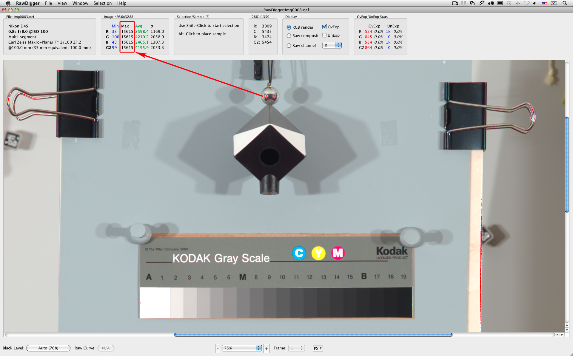
Figure 6. A shot of Q13 opened in RawDigger
The values for those blown-out areas reach the maximum available for the camera at the given ISO, so we can take the maximum value from the statistics, this value being 15615 (you should not expect it to be exactly 16383, 2^14-1).By the way, we are sure that the areas are blown out also because the readings in all 4 channels, RGBG, are not only high, but very close to each other too – they hit the hard limit.
This shot was exposed in such a way, that the brightest patch is close to clipping. Making a selection over the "A" patch we can see it is 14209.4, which, according to formula (5) and taking into the account the gamma for the raw data = 1 (the raw data is linear), is:
| log2(14209.4/15615) ≈ –0.14 EV from clipping (1/6 EV is ≈0.17 EV) |
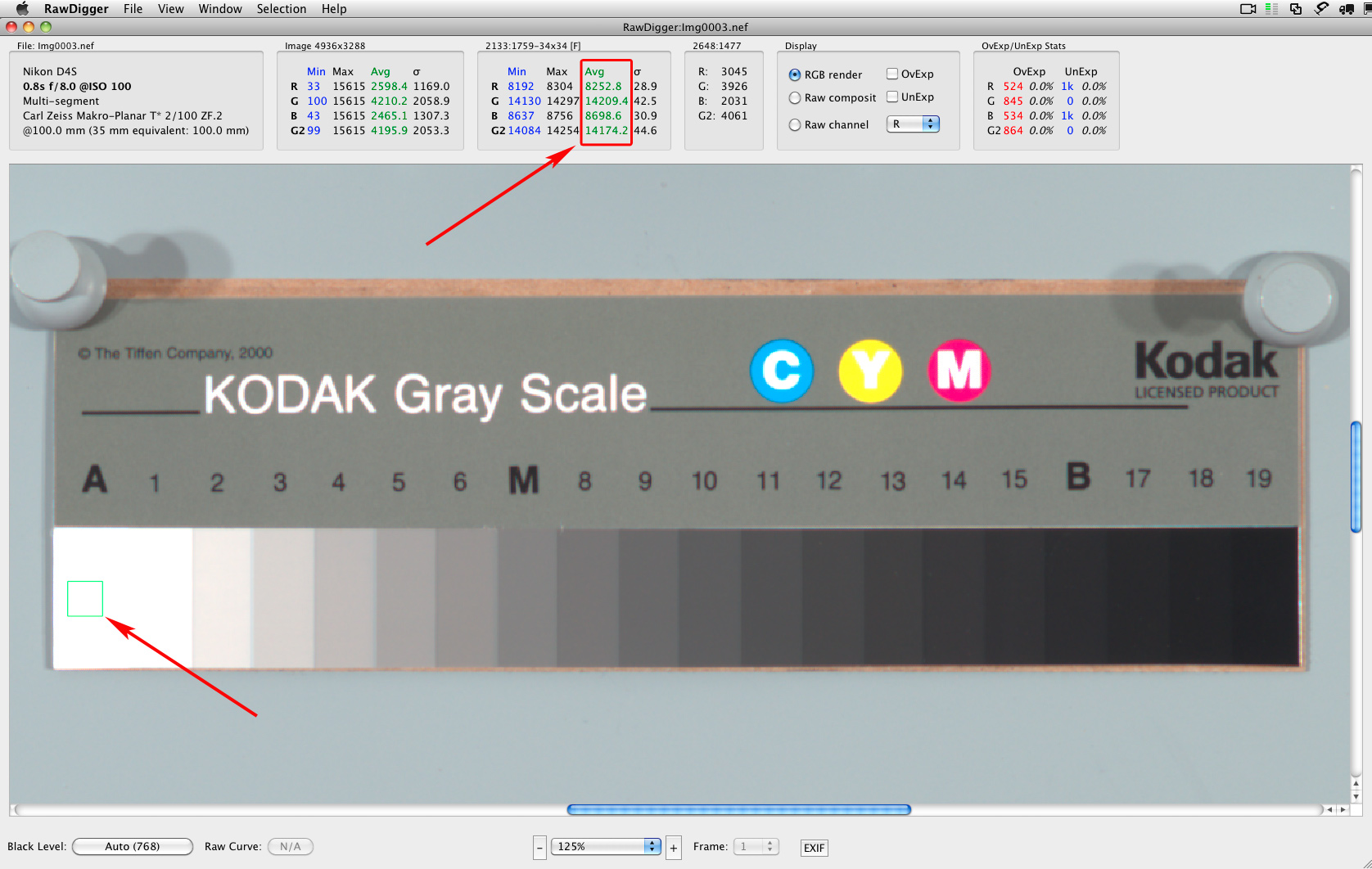
Figure 7. Q13. Patch "A" - selection and data numbers>
Next, let's check the value of the "M" patch with RawDigger. Selection over the "M" patch results in an average value of 2755.8.
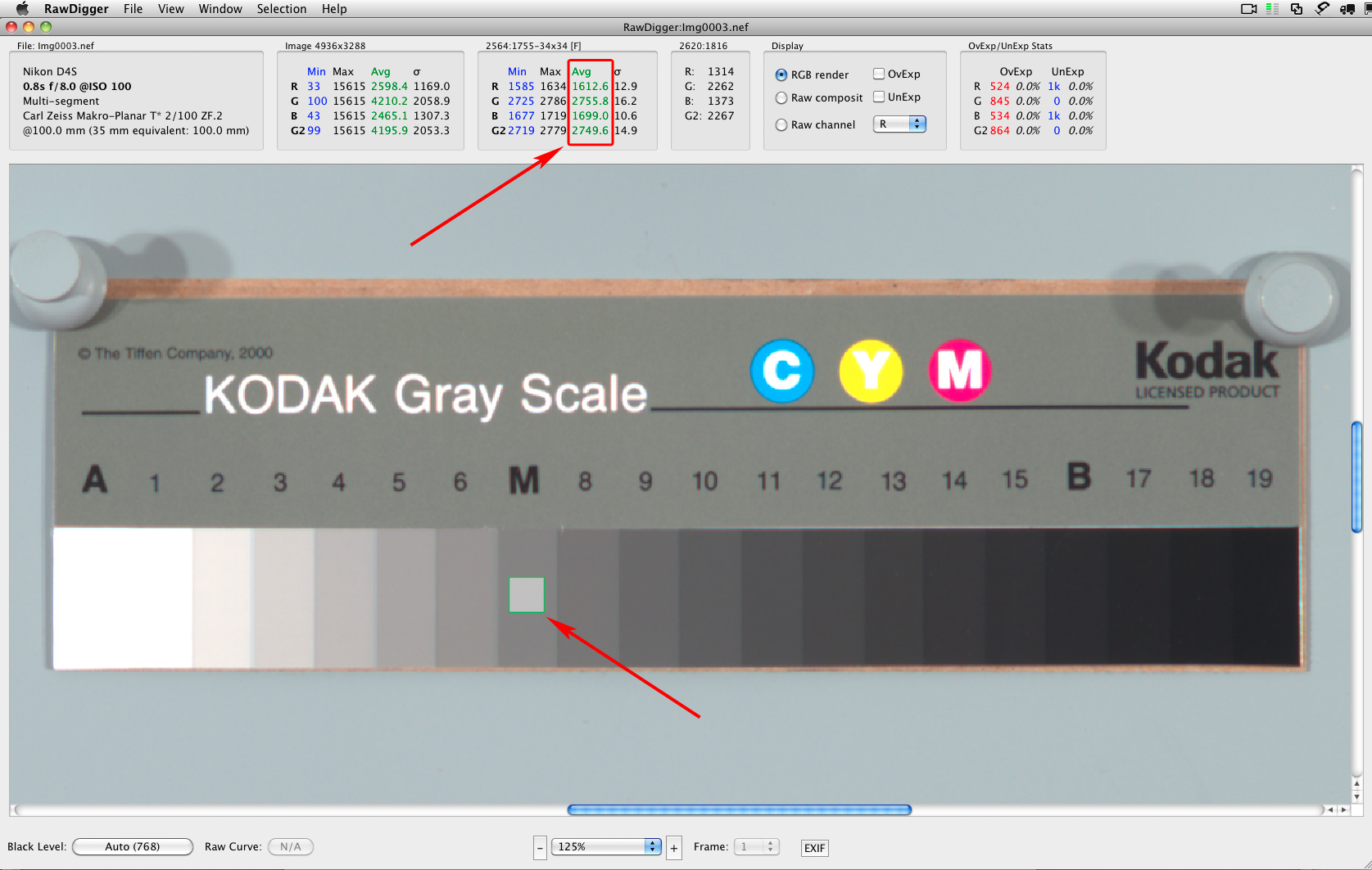
Figure 8. Q13. Patch "M" - selection and data numbers
As we can see, the "M" patch on the shot is very close to the academic mid-tone of 18% and to Kodak's formulation of 17.78% (see above) - from formula (4); again, using gamma=1 since it is linear raw data, we have:
| 2755.8 / 15615 *100% = 17.65% |
As it was already mentioned, ISO standard 12232 calls for the midpoint on a rendered image to be 18% grey, corresponding to the value of 118 in 8-bit (0..255) sRGB within the margin of ±1/3 EV.
To convert this interval into photographic stops we use formula (5) with gamma 2.2:
| log2((118/255)^2.2)±1/3 EV = -2.45 ± 1/3 EV |
It means that in photographic stops the interval for the midpoint is between -2.12 EV and -2.78 EV
To get back to RBG values we have to repeat the same calculations in reverse, and, to spare you the details, the result is that we should expect midpoint to be between 105 and 130, accounting for ±1/3 EV tolerance the standard suggests.
Now, let's open the image in Adobe CameraRaw and check the value of “M” patch.
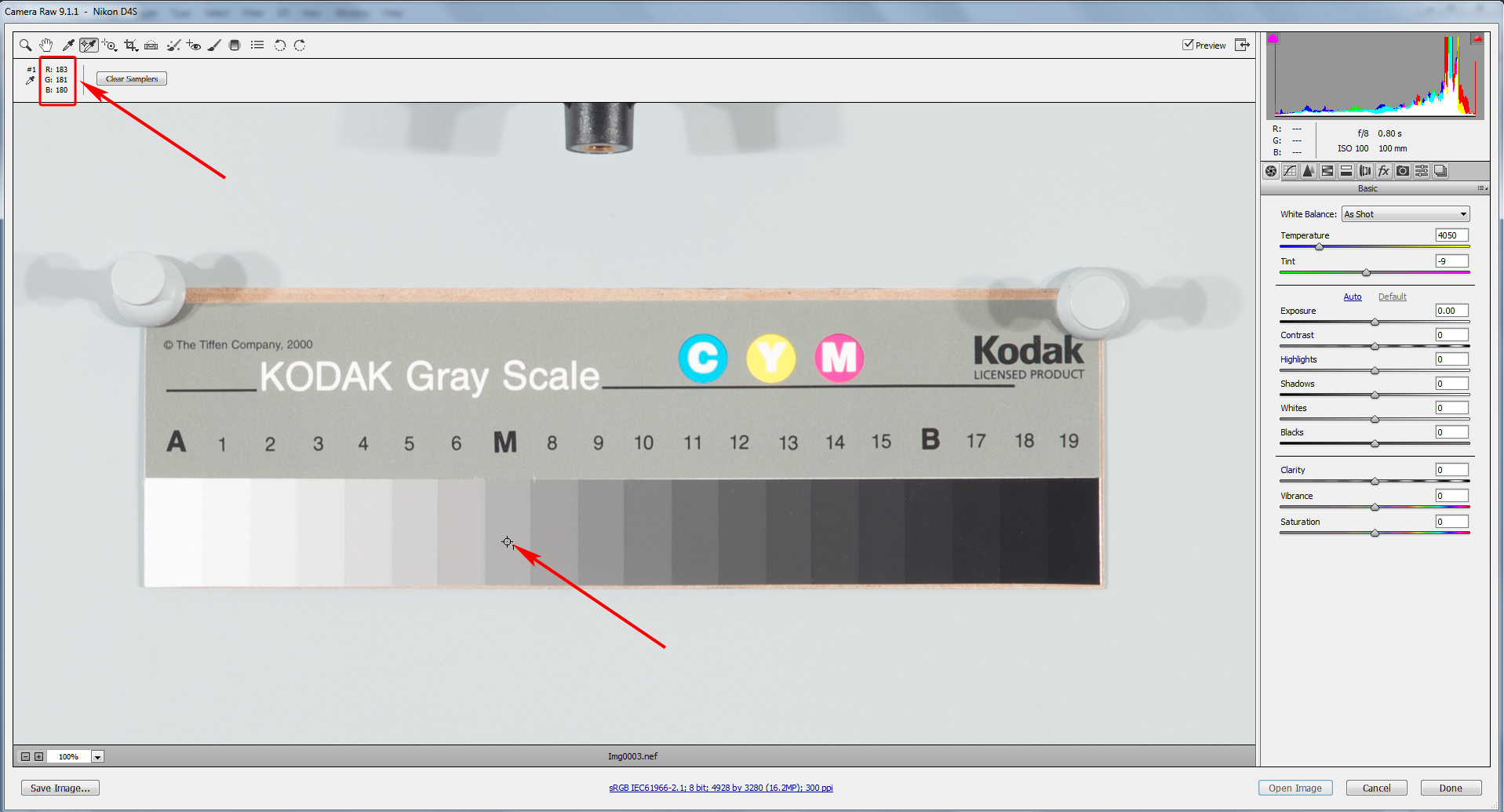
Figure 9. Q13 in ACR, "M" patch value
It is 181 in the Green channel in sRGB, pretty far from the midpoint (if you are using Lightroom, you can turn SoftProofing on and set it to proof to sRGB to see the RGB numbers on a 0..255 scale). But how far is it in photographic terms, that is to say in EV?
Lets make some calculations, taking into account that the standard speaks of gamma = 2.2 for sRGB:
The standard calls for 118 RGB for "M" patch, so according to the standard the reflectivity on "M" patch should be (using formulas (4) and (5)):
| ((118/255)^2.2)*100% ≈ 18.4% | |
| log2((118/255)^2.2) ≈ -2.44 EV (2.44 EV down from clipping) |
On our shot the "M" patch is 2755.8 in Green channel (see Figure 8); the maximum value is 15615; and gamma=1, so the reflectivity of "M" patch from the raw data is (using the same formulas):
| (2755.2/15615)*100% ≈ 17.65% | |
| log2(2755.2/15615) ≈ -2.5 EV (2.5 EV down from clipping) |
as we have already mentioned, the "M" patch is very close to the academic mid-tone of 18% and to Kodak's formulation of 17.78%,
After raw conversion, we got 181 RGB for the "M" patch:
| (181/255)^2.2)*100% ≈ 47% (instead of 18%) | |
| log2((181/255)^2.2) = -1 EV (1 EV down from clipping, instead of 2.5 EV) |
This means that the mid-tone is bumped by about 1.5 EV! No wonder higher mid-tones start to look featureless: they are heavily compressed through a very long and flat shoulder of the default tone curve.
This actually means that if you were to try and expose in such a way that the defaults in a raw converter place a mid-tone where it belongs on the default rendition, you might end up underexposing by more than 1 EV -- just start decreasing the value of Exposure and watch how 118 in the green channel appears when the slider is at -1.2 EV.
This might be not so detrimental when light is aplenty and you are keeping ISO low, but in dim light with exposure going down, and ISO going up, you will heavily deplete the camera's dynamic range.
Practical Part: How You Can Override Default Adjustments
Lets see if we can change the defaults in such a way that no hidden brightening will happen during raw conversion.
Such defaults are easier to set using Process Version 2 (abbreviated as PV 2, previously known as Process Version 2010 or PV 2010). Let's switch to it. To do so, press the camera icon to activate "Camera Calibration" tab and select PV 2 (2010) from the "Process" drop-down. Default settings are now: Brightness = 50, Contrast = 25, Blacks = 5, and Medium Contrast curve. So, one can immediately see that some adjustment have been made to a shot.
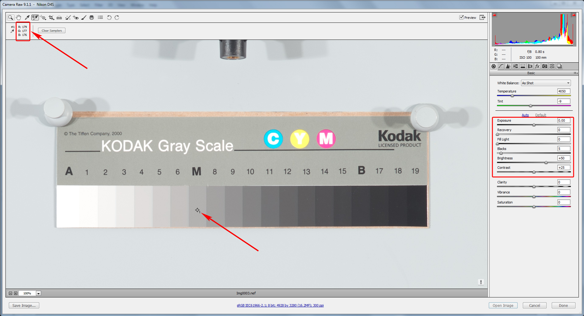
Figure 10. Q13. ACR, PV 2 (2010)
Just on a side note: selected point of the "M" patch with the default render of this shot Q13 in ACR set to PV 2 (2010) has value 177 in Green channel, while for the default render with PV 3 (2012) the value for the very same point was 181.
As some of our readers may know, Dan Margulis advocates starting with the zeroed-out rendition; and only then adjusting the sliders to choose the proper settings for conversion; or, better yet, converting with zeroed-out settings and continuing in Photoshop.
Setting Blacks, Brightness and Contrast sliders all to zero, and dropping the curve to Linear, we see that the "M" patch value now becomes 129, that is, according to the standard, in the ballpark for a mid-tone. Only on the upper margin of it, however.
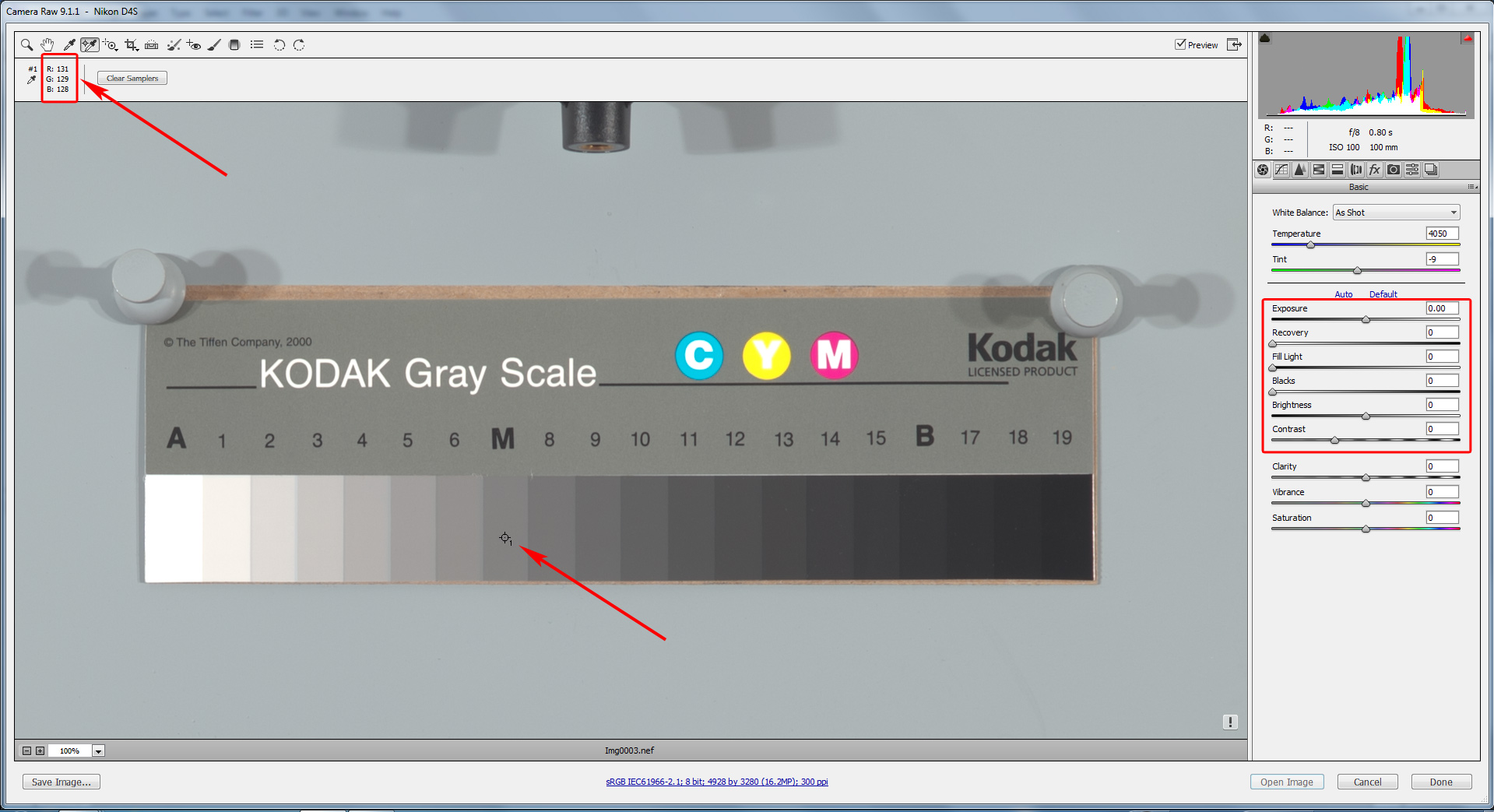
Figure 11. Q13. ACR set to PV 2 (2010), defaults are zeroed out
Switching back to PV 3 (2012), you can save the resulting settings and use them for zeroed-out renditions - as you can see, now "M" patch has value 133 in Green channel, placing it very close to where mid-tone belongs.
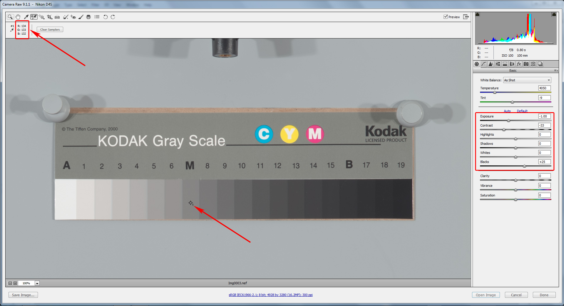
Figure 12. Q13. ACR, back to PV 3 (2012)
Nevertheless, for the PV 3 (2012) we are slightly above the standard upper margin, and for PV 2 (2010) we are just a little below it. Why? Remember when we discussed the silent/hidden exposure compensation Adobe are applying? This "BaselineExposure" (BLE) happens to be 0.25 EV for Nikon D4s for this ISO. Subtracting it from the Exposure, we see the sRGB number in the green channel dropping to 119 for the PV 2 (2010) with zeroed out defaults.
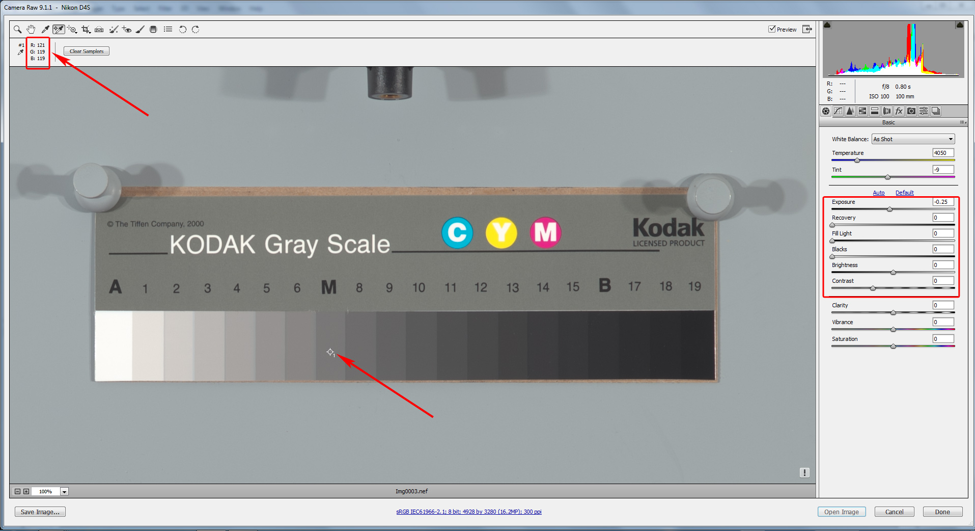
Figure 13. PV 2 (2010), zeroed-out defaults, 0.25 BaselineExposure subtracted
… and 123 for PV 3 (2012) with zeroed-out defaults.
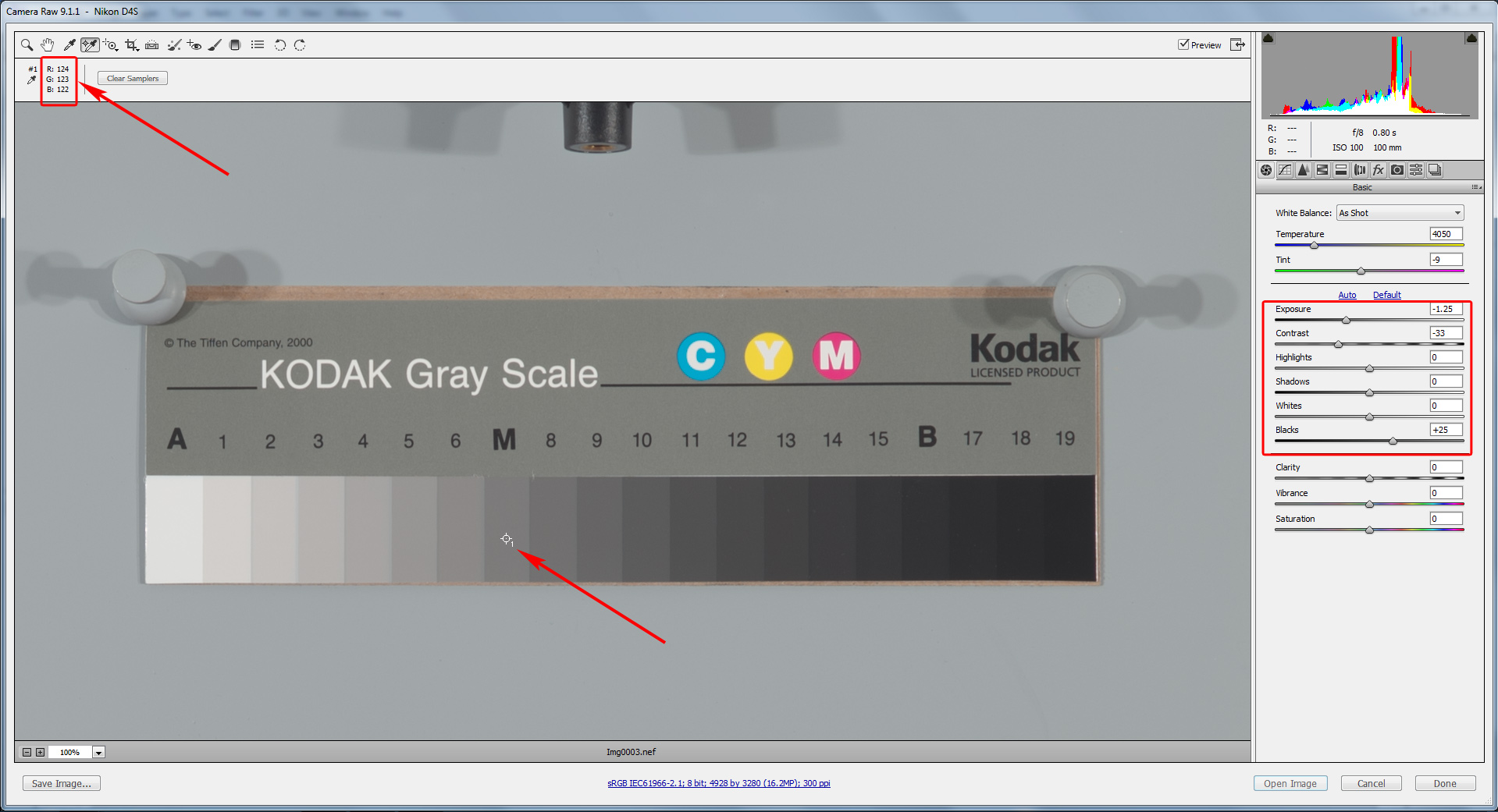
Figure 14. PV 3 (2012), zeroed out defaults, BaselineExposure subtracted
Voilà! Now, with these settings, we have the mid-tone placed correctly, within the tolerance allowed by the standard.
Some Words About BaselineExposure
We have already touched upon this subject a year ago in the article "Adobe Silent Exposure Compensation".
Another way to look at BaselineExposure is this: BaselineExposure indicates the difference between clipping in the raw converter and clipping in the raw itself. BaselineExposure is the amount of EV to which the highlights can be brought back (un-clipped) before "highlight recovery" (that is, the interpolation that reconstructs the clipped channels based on the channels that are not clipped) kicks in.
Referring to certain cameras, some folks say that those cameras allow one to "restore clipped highlights" better. But those highlights they are restoring are not clipped in raw, they are clipped in a raw converter, that is no restoration happens, just smoke and mirrors. The price for this "feature" is straightforward underexposure, resulting in more artifacts and noise - the lower the camera metering system is calibrated, the lower the exposure, the more headroom in highlights there is for "restoring", and the higher the BaselineExposure number.
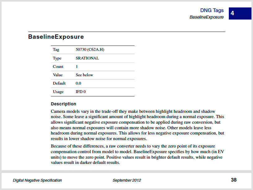
Figure 15. Adobe Digital Negative Specification, version 1.4.0.0., June 2012, page 38
But I digress...
To be sure of what is happening, we'll use a synthetic dng with simulated 16-bit Q13 step wedge. The simulation is based on the above-mentioned Kodak formulation; "A" is 0.05D, and each next step adds 0.1D (in other words, the step is 1/3 EV). The BaselineExposure for this DNG is 0, because of how we created that synthetic dng.
Using superposition of formulas (3) and (5) we will get that RGB value for every patch calculated based on its density:
| RGBpatch = RGBMax/10^(Dpatch/gamma) | (6) |
Based on this formula we can calculate RGB values for every patch of the Q13 for RGB color space with various gamma values.
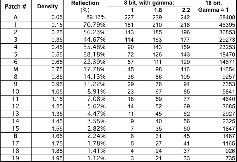
Figure 16. RGB values for Q13 patches
Now we open our synthetic dng with simulated 16-bit Q13 step wedge in RawDigger,
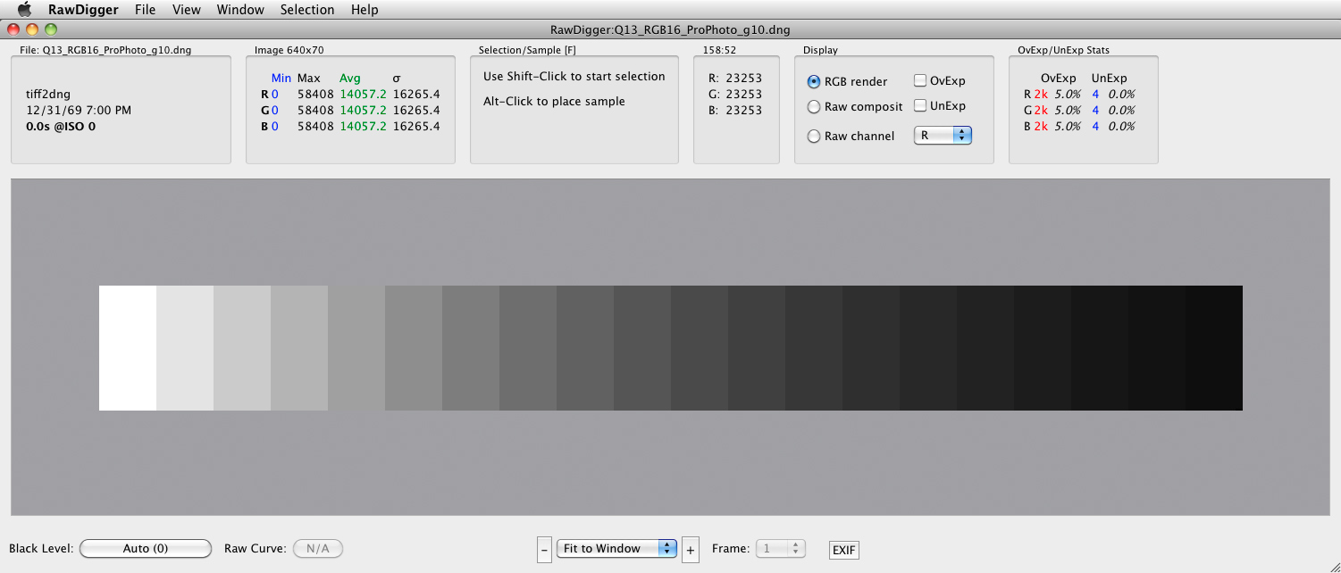
Figure 17. Simulated Q13 step wedge
… make a selection grid,
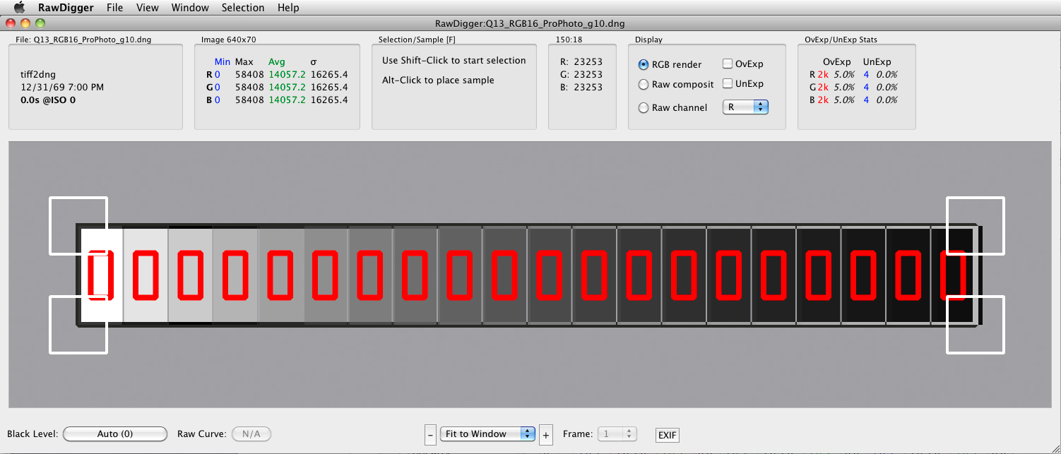
Figure 18. Simulate Q13 with grid selection
… and save selection’s RGB values as a table (Excel-compatible .CSV):
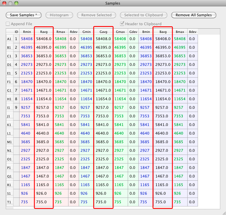
Figure 19. 16-bit Q13 RGB values
Comparing the numbers calculated (Figure 16, last column – since we have 16-bit linear data) to the numbers in RawDigger (Figure 19) you can see the synthetic dng step wedge is correct.
Now, if you open our synthetic dng in ACR (using PV 2 /2010/ as more obvious and precise), zero out the settings, place color samplers to 9 patches (unfortunately, ACR allows only up to 9 color samplers at once) and compare the numbers with the table on Figire 16 (please use the appropriate gamma column, 1.8 for ProPhoto, 2.2 for AdobeRGB and sRGB; the numbers agree best for ProPhoto RGB and AdobeRGB due to true sRGB not exactly being the gamma 2.2 space, which affects mostly shadows), you will see that the numbers are very close to what they should be.
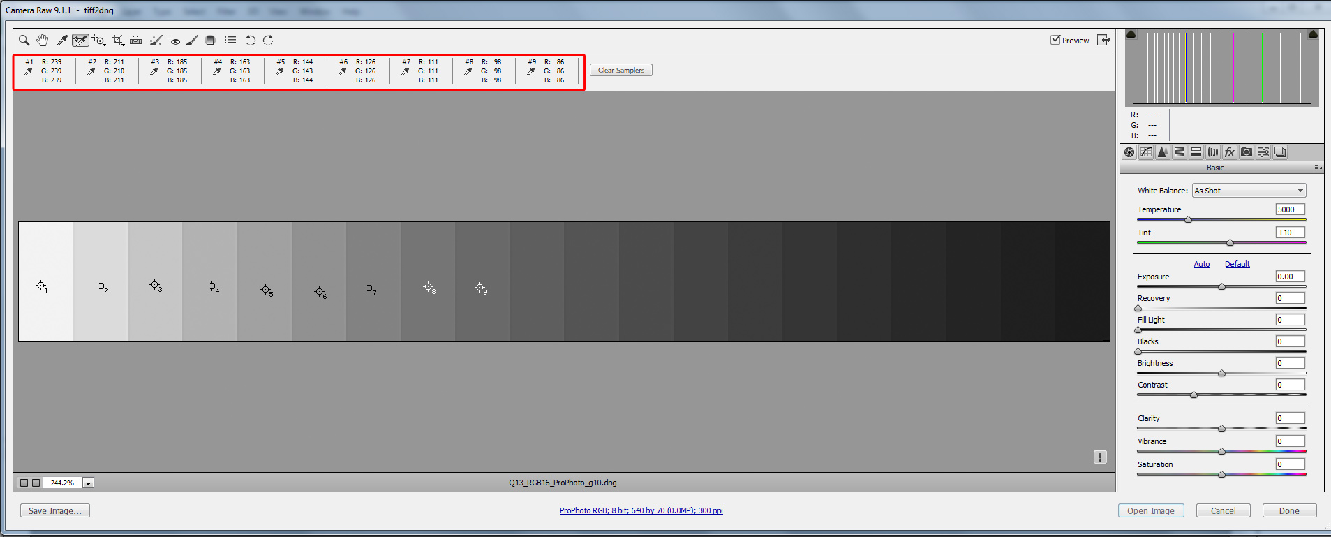
Figure 20. Simulated Q13 in ACR, ProPhoto RGB, gamma 1.8
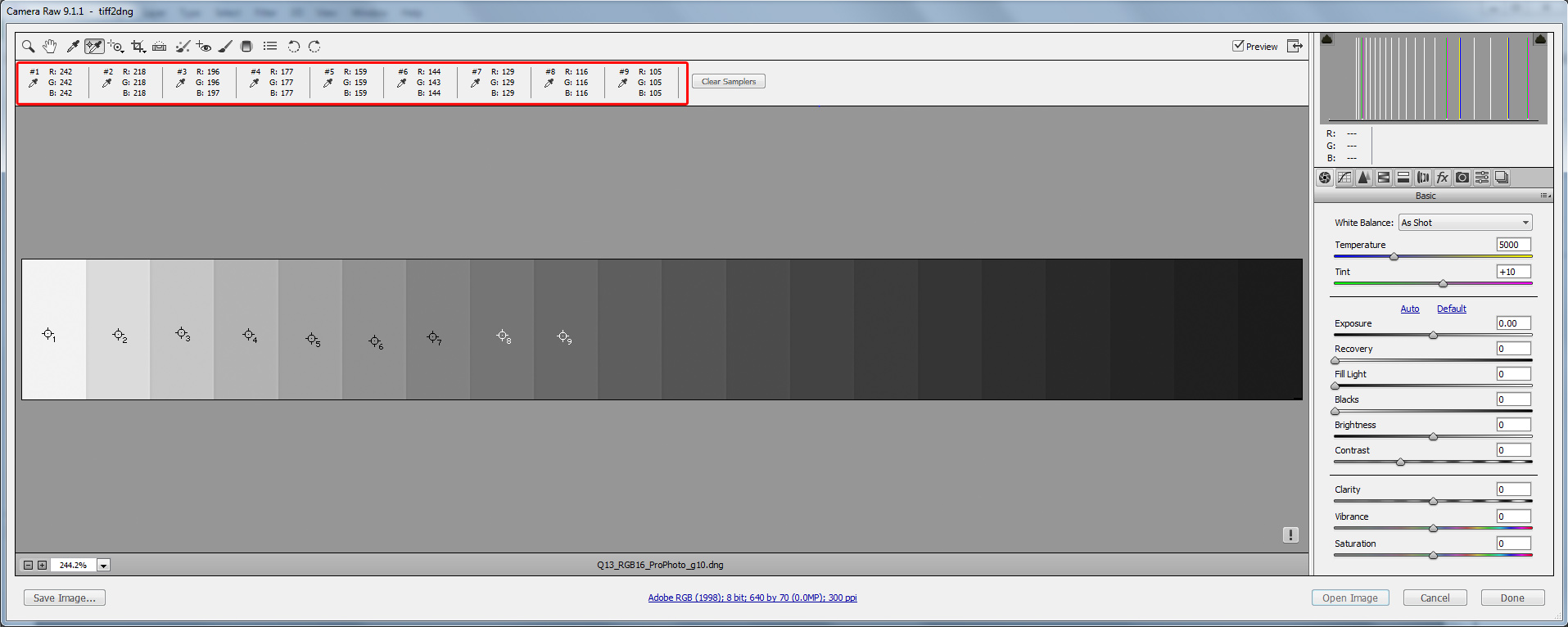
Figure 21. Simulated Q13, ACR, AdobeRGB, gamma 2.2
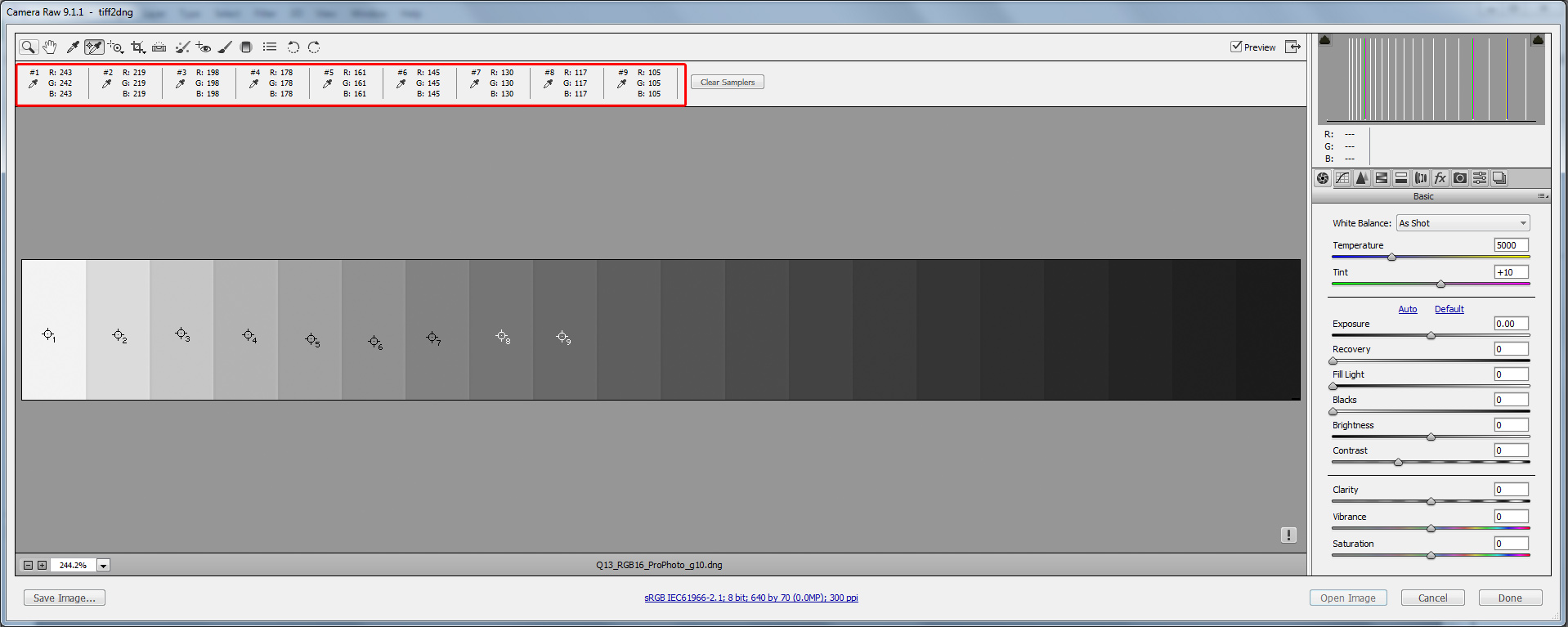
Figure 22. Simulated Q13, ACR, sRGB
It proves our statement that after we zeroed-out defaults in Adobe raw converter we are getting accurate scene reproduction, within the BaselineExposure compensation.
In the next article we show you how to calculate BaselineExposure for your camera using RawDigger.
The Unique Essential Workflow Tool
for Every RAW Shooter
FastRawViewer is a must have; it's all you need for extremely fast and reliable culling, direct presentation, as well as for speeding up of the conversion stage of any amounts of any RAW images of every format.

Now with Grid Mode View, Select/Deselect and Multiple Files operations, Screen Sharpening, Highlight Inspection and more.
11 Comments
Capture One
Submitted by Alphonse PHILIPPE (not verified) on
HI,
How to apply this in Capture One ?
Thanks
A. PHILIPPPE
Dear Sir:
Submitted by LibRaw on
Dear Sir:
You can start with shooting some gray step wedge (you can do it with a bracketed exposure of some gray card, too -- just more shots and more work needed) and comparing actual raw values obtained with RawDigger with the values CaptureOne renders. It is important to use your camera. When you will have the shots, we can help you further, our e-mail is support@rawdigger.com
When you talk about
Submitted by Marcin (not verified) on
When you talk about overriding default adjustments in LR/ACR and "zeroing things out" (as advocated by Dan Margulis) you do not mention the tone-response curve hidden in the input colour profile. The Adobe Standard profile for the cameras I've tested ships with some S-shaped curve as well -- wouldn't that affect the calculation of the Baseline Exposure? Thanks.
Dear Sir:
Submitted by LibRaw on
Dear Sir:
You can replace that curve with a straight one if you wish so; in Process Version 2010 (PV2010) it does not affect the baseline exposure, an if that value of baseline exposure is determined, you can use it in PV2012 as well. But my personal preference is replacing the curve, maybe I will add a short instruction how to do that.
Thanks for the answer. I have
Submitted by Marcin (not verified) on
Thanks for the answer. I have modified the Adobe Standard .dcp profile for my cameras within the Adobe DNG Profile Editor, where you can use the linear curve. Is that how you do it?
Dear Sir:
Submitted by LibRaw on
Dear Sir:
One of the ways to check what curve you have in a DCP is with free exiftool. The command line is:
> exiftool -ProfileToneCurve -b profile_name.dcp
Great, thanks.
Submitted by Marcin (not verified) on
Great, thanks.
Suppose you want to create an
Submitted by Wouter Van Der ... (not verified) on
Suppose you want to create an extended shoulder to store the highlight information and that you want to achieve 6.5 stops measured from middle grey up to clipping point. To stay true to scene referred contrast/gamma we thus have a difference of 2.5 stops between the white patch and the middle grey patch, as specified by this post. This leaves room to push 3 stops into the highlight shoulder in my case (+ possible additional highlight reconstruction information).
My question is: starting from the green channel's full saturation point, where should I map the white patch? In your example you suggest around 0.15 EV from full saturation but that means I would have to cram 3 stops into a space of 0.15 EV. I think this would remove all the detail and be rendered as white on a display (sRGB/Rec.709). I want to achieve a smooth rolloff into pure white without losing too much detail nor creating abrupt, harsh transitions into white.
So where would you advise me to put the white patch?
I was thinking of putting it around 2 stops over middle grey. This would then mean that the 3 stops highlight information would be crammed into a space of about half a stop, maybe a little more (0.5 EV + 0.15 EV)?
Does this seem like a reasonable thing to do?
Similar for the toe: where do I place the black patch of the test strip before the tones start to roll off into the toe, into complete blackness?
The goal is to get to a tone map that is similar to how film scans used to be transformed for sRGB display.
And another question: what comes first? Chroma mapping or tone mapping? White balance before or after the tone mapping?
Any help would be greatly appreciated! Thank you!
We need an updated article on
Submitted by viktor (not verified) on
We need an updated article on this for lightroom classic cc! 👍
If the standard Adobe RAW
Submitted by Nik (not verified) on
If the standard Adobe RAW converter is so off, why do they implement it?
amazing photography
Submitted by Romel Adhikary (not verified) on
Wonderful post. I am involved in professional photography, and required a good converter. I am already using the converter. How to apply this in Capture One?
Add new comment