
Submitted by lexa on
Study of the highlight clipping using RawDigger histogram
It is useful to know how to determine practical clipping point for at least two reasons: the most common is that we need to know clipping point to determine the headroom in highlights and tune the camera settings to provide more reliable overexposure warning (“blinkies”); another one is dynamic range analysis (signal-to-noise ratio, SNR), and measurements of utilized well capacity (full well capacity, FWC, is seldom used in modern cameras).
Different cameras, even if based on the same sensor, may render extreme highlights around the clipping point differently; and differently, even with different values of clipping points, depending on ISO setting. It is important to recognize the look and calculate the practical clipping point, which is not always the same as the maximum raw value. Here we will try to demonstrate the typical “looks” of the histogram of the clipping zone.
Any curved metal or glass surface is a good source of specular highlights. In our case, it is what we want as we will be analyzing how the clipping exhibits itself on the shots like these from Imaging Resource:
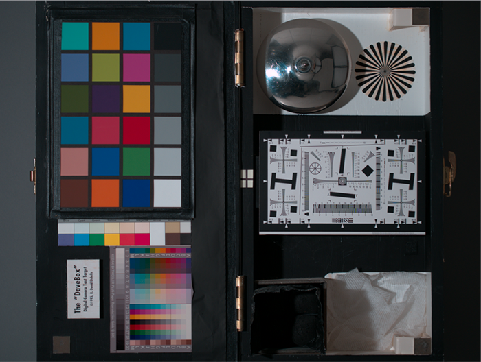
Figure 1. "Davebox" Test Target
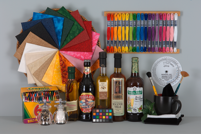
Figure 2. Still Life
A shiny metal ball, or any metal bowl, is also a good target to inspect highlights and clipping. Having dark background behind the shiny surface helps to isolate highlights on the histogram. If you are anticipating performing dynamic range analysis having a black trap in the same shot saves time (you can make a black trap yourself, see http://www.imatest.com/docs/veilingglare/ #target, or use the Datacolor SpyderCUBE, as we did below).
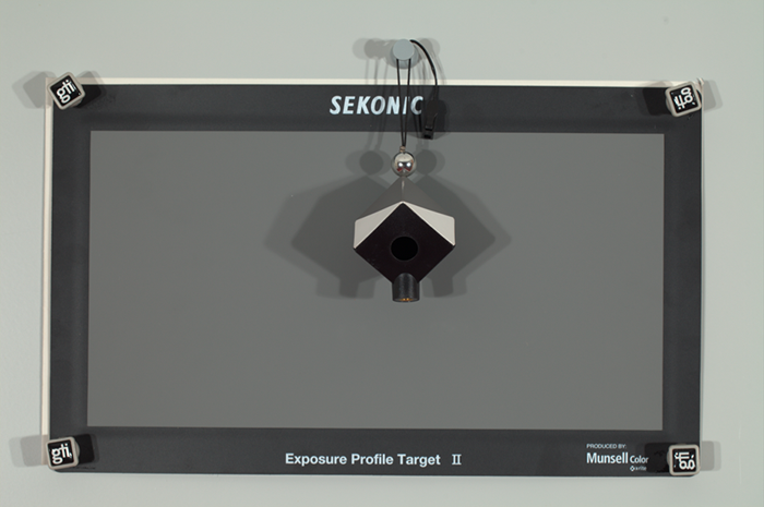
Figure 3. Datacolor SpyderCUBE
We are going to open these shots, made by different cameras, in RawDigger. OvExp checkmark in the Display section causes a red overlay to appear over the blown highlights, similar to the “blinkies” in-camera overexposure indication. To make these small areas more noticeable we additionally placed red rectangles over these areas.
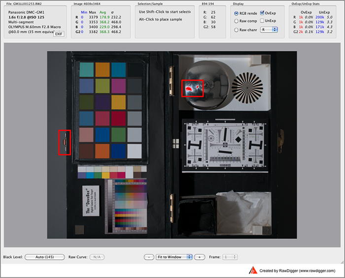
Figure 4. "Davebox" Test Target opened in RawDigger with Overexposure Indication on
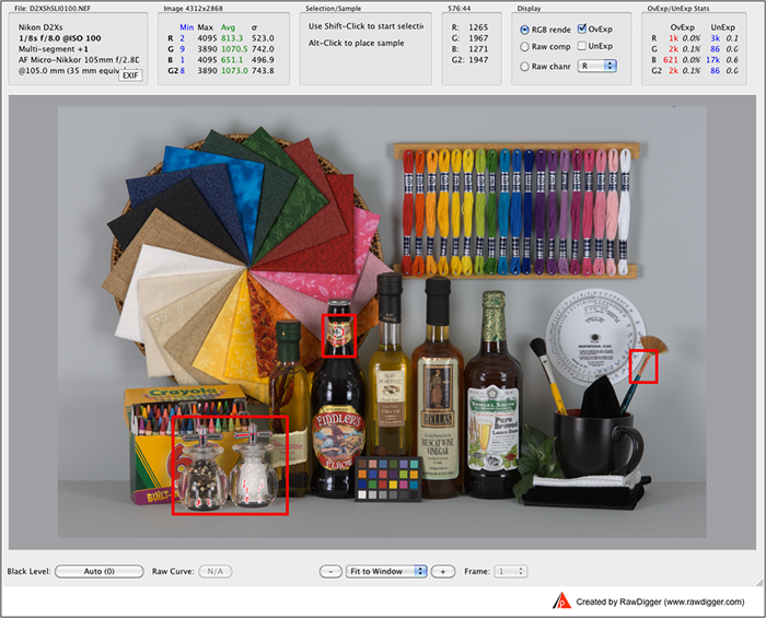
Figure 5. Still Life opened in RawDigger with Overexposure Indication on
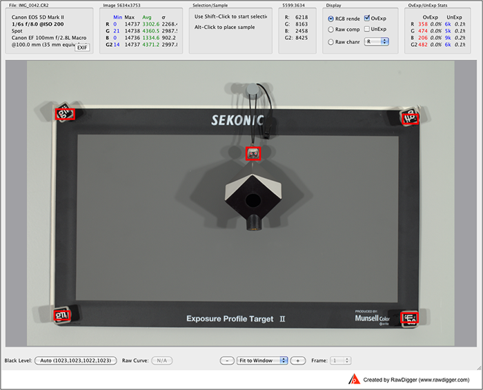
Figure 6. Datacolor SpyderCUBE opened in RawDigger with Overexposure Indication on
… and look at their histograms.
To look at histograms’ structures in more detail, let’s switch on the “Log scale” on the Y-axis, and for starters turn on “Linear X-Axis” and check Auto both for X-axis and Y-axis range:
Upd: Francisco Disilvestro made an important point:
We'd like to add to check that you have the "Masked Pixels" option unchecked in the Preferences -> Display options.
Some cameras have reference pixels hard-wired to min an max numeric levels in the masked pixels area, which will show as a spike in the histogram where there should be none. This is easy to note in cameras that have different blown out levels for different channels, such as some Nikon models. In those cases, you will see a spike at blown out level and then another small spike at the maximum numerical value (depends on bit-depth)
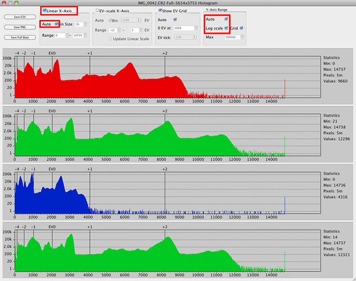
Figure 7. Histogram – full range, log Y-axis scale
For even more detailed view we reduce the displayed range along X-axis so that it will include, more or less, only the area of highlights. Switching off “Auto” in the “Linear X-Axis” section, we can set the left margin of the range close to the structure in the highlights. Now we can set the bin size to 1. We will be referring to this set of actions as to zoom in to the highlight portion of the histogram.
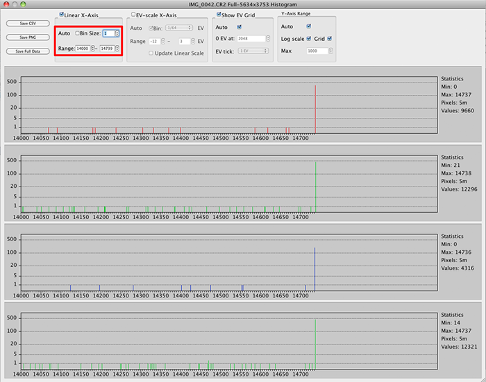
Figure 8. Histogram – “zoom in” onto blown highlights
For overexposed shots with blown-out highlights the extreme right of the histogram usually takes one of following typical shapes:
- a two-slope structure, which resembles the Empire State Building,
- a two-slope structure, resembling a bell,
- a one-slope structure, which brings to mind a wave hitting the wall,
- a spike,
- a hybrid structure (may be different in every color channel)
1. The “Empire State Building” as displayed in log scale Y-axis mode (a typical example would be SONY cRAW/ARW2):
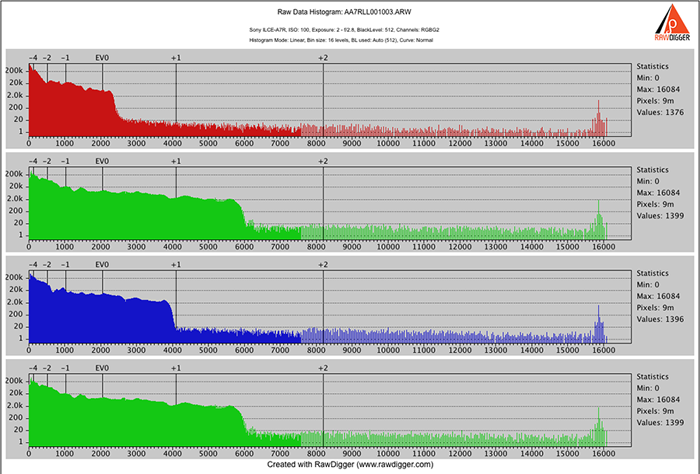
Figure 9. Sony A7R. Full range histogram for the “Empire State Building” – type structure
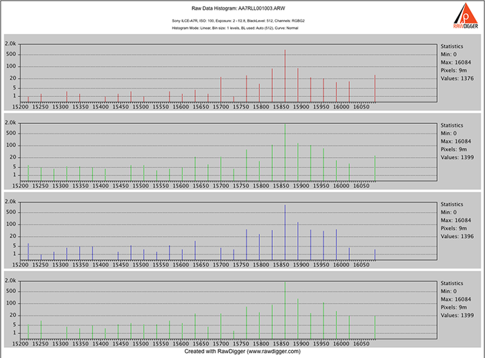
Figure 10. Sony A7R. Zoom to the “Empire State Building” structure
2. A “bell” as displayed in log scale Y-axis mode (Canon):
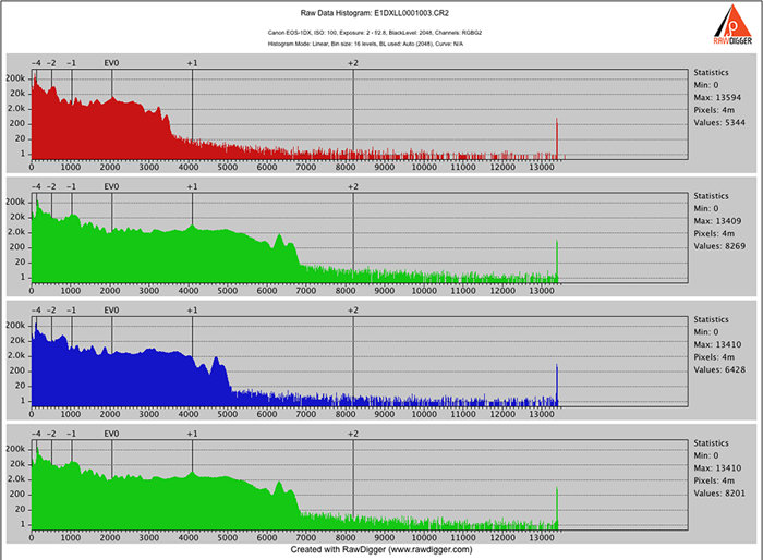
Figure 11. Canon EOS-1DX . Full range histogram for a “bell”- type structure
For those wondering why we classified this as a bell-shaped rather than an the “Empire State”, this is why:
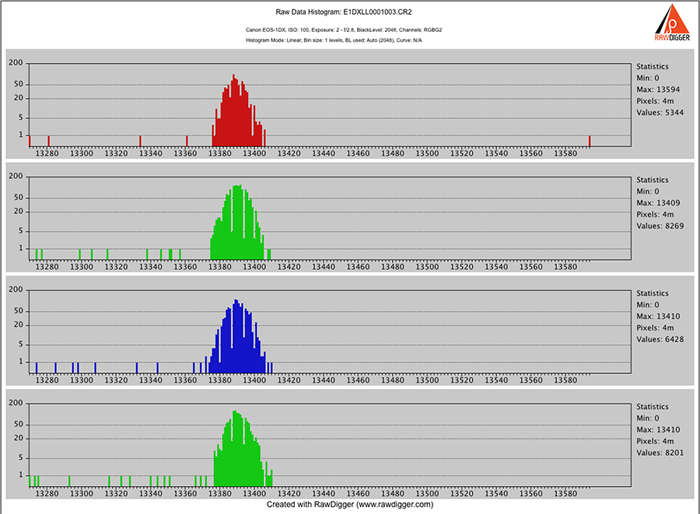
Figure 12. Canon EOS-1DX. Zoom to the “bell” structure
3. A “wave hitting the wall” as displayed in log scale Y-axis mode (Sigma):
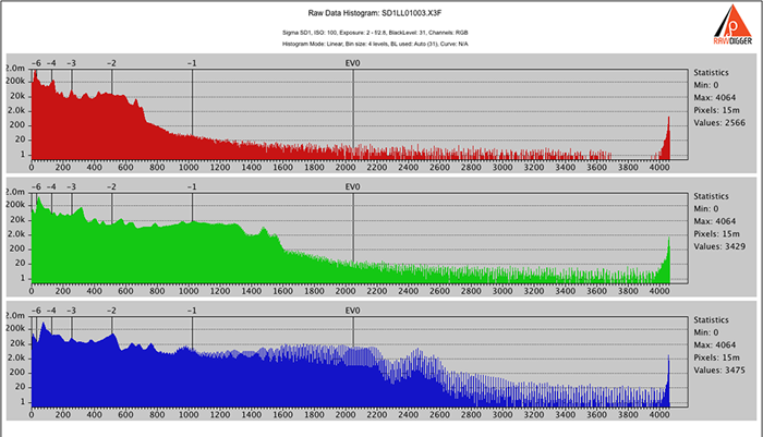
Figure 13. Sigma SD1. Full range histogram for a “wave hitting the wall” - type structure
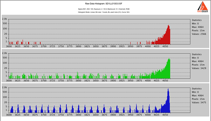
Figure 14. Sigma SD1. Zoom to the “wave hitting the wall” structure
4. A “spike” as displayed in log scale Y-axis mode (Pentax, Leica, Samsung)
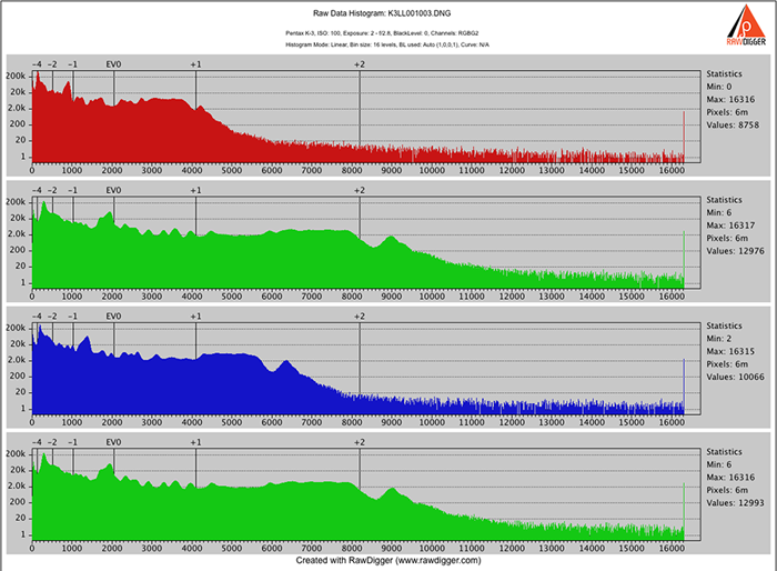
Figure 15. Pentax K-3. Full range histogram for a “spike”- type structure
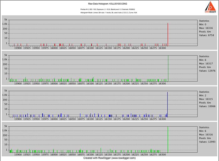
Figure 16. Pentax K-3. Zoom to the “spike” structure
5. A hybrid structure as displayed in log scale Y-axis mode (a typical example would be shots from Fujifilm)
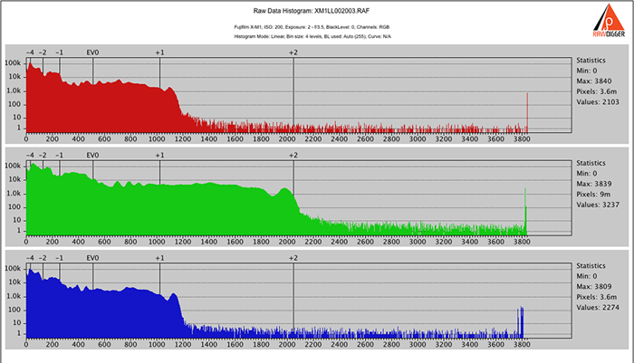
Figure 17. Fujifilm X-M1. Full range histogram for a hybrid structure
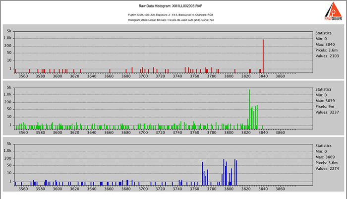
Figure 18. Fujifilm X-M1. Zoom to the hybrid structure
Some cameras, such as Canon and a few Panasonic cameras have a certain peculiarity – their maximum (that is a clipping point) changes depending on the ISO setting.
Take for instance this particular histogram of a shot from a Panasonic GM1 at ISO 125:
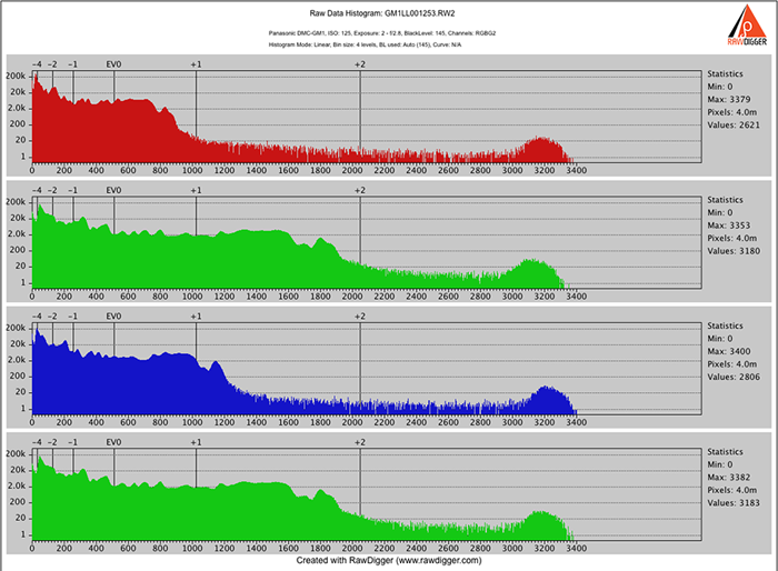
Figure 19. Panasonic GM1. ISO 125 - full range histogram with a “bell”- type structure of blown-out highlights
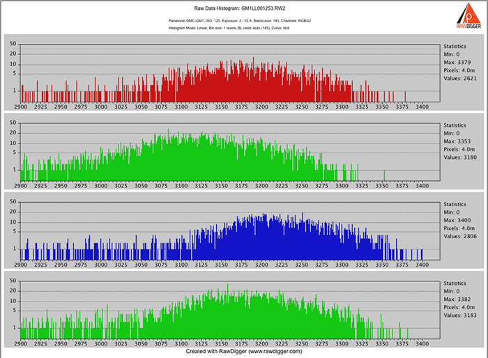
Figure 20. Panasonic GM1. ISO 125 – zoom to the “bell” structure on the histogram
This seems normal, in and of itself, but, if one were to take a look at the shot at ISO 400…
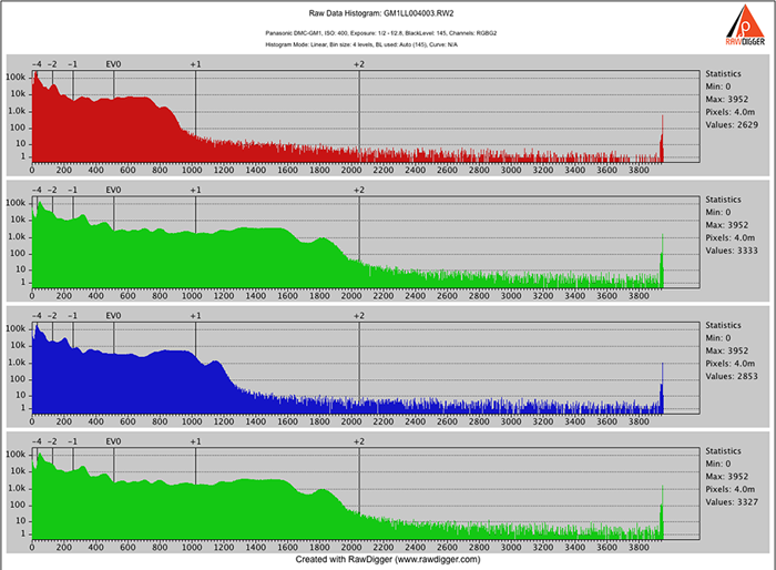
Figure 21. Panasonic GM1. ISO 400 - full range histogram with a “wave hitting the wall” – type of blown-out highlights
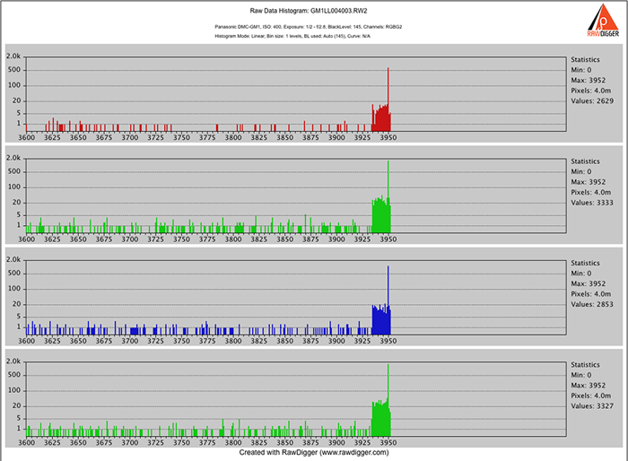
Figure 22. Panasonic GM1. ISO 400 – zoom to the “wave hitting the wall”
…It becomes plainly evident that the maximum has shifted at least 500 levels to the right, and the bell-shaped curve is no longer there.
n certain cases, the «blown-out highlight» histogram’s structures will not be aligned vertically, meaning that the center values of the structures will be different for different channels.
Most often, this is the indication of color channels (white balance) preconditioning, like the one Nikon is using on of their cameras since D2X (D5300 and D3300 are two recent exceptions).
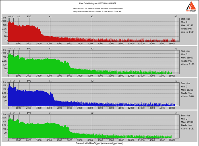
Figure 23. Nikon D800. Full range histogram - color channels preconditioning
This is as it looks in full-range, and this is how it looks if we zoom in closer. We see that maximums are different for different channels:
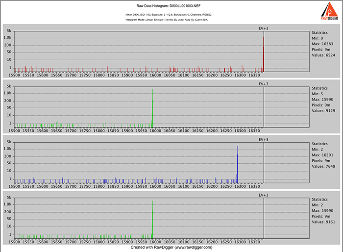
Figure 24. Nikon D800. Zoom to blown out highlights - maximums are different for different channels
Cameras where color channel preconditioning is used are recognizable by the regular one-pixel gaps in the histograms of red and blue channels (sometimes, additionally, they have different clipping points for red, blue, and both green channels, as on fig.24). This is because of how the preconditioning is implemented – it is digital multiplication of data in red and blue channels by a number slightly higher than 1, applied before the data is written into a raw file.
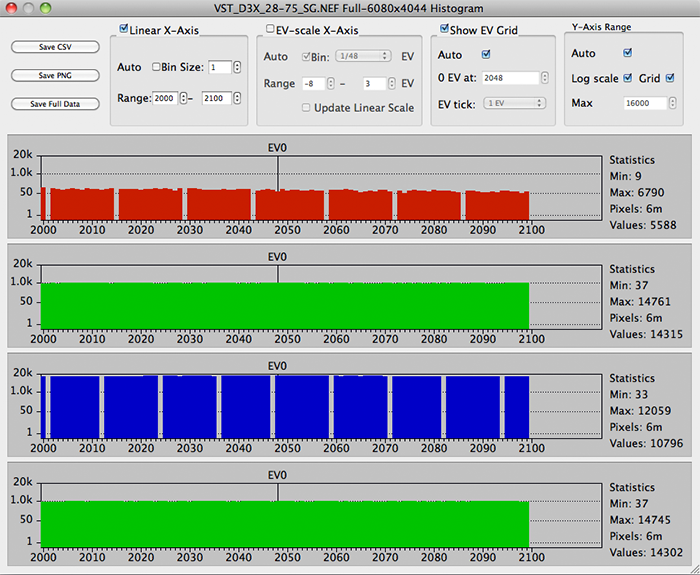
Figure 25. Nikon D3X. Color channels preconditioning zoomed in.
Which value should be considered as practical maximum?
The conservative approach is to consider the value that starts the overexposure “structure” to be the maximum, as the higher values are mostly pattern and processing noise. For “hit-the-wall” and “spike” types of highlight structures, it is the spike itself. However for something like we have on fig.22, which is not a pure “hit-the-wall”, the clipping starts at 3935.
So, if we return to the histogram shown on figs. 9 and 10 for Sony A7R, we will see that here the peak value is 15860, while the bulk of the structure starts at 15635.
Now we can go into Preferences and, following the conservative approach, enter this second number to Overexposure Detection section in Manual level all channels field.
Note: If your camera is one of those with white balance pre-conditioning, you will need to enter per-channel values in Manual per channel section R, G, B, G2 fields
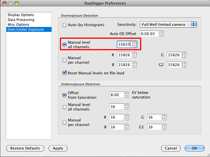
Figure 26. RawDigger Preference menu. Over/Underexposure settings
Now we can hit Apply and inspect the main view. If you have done everything above correctly, you will have a very accurate display of the overexposed areas.
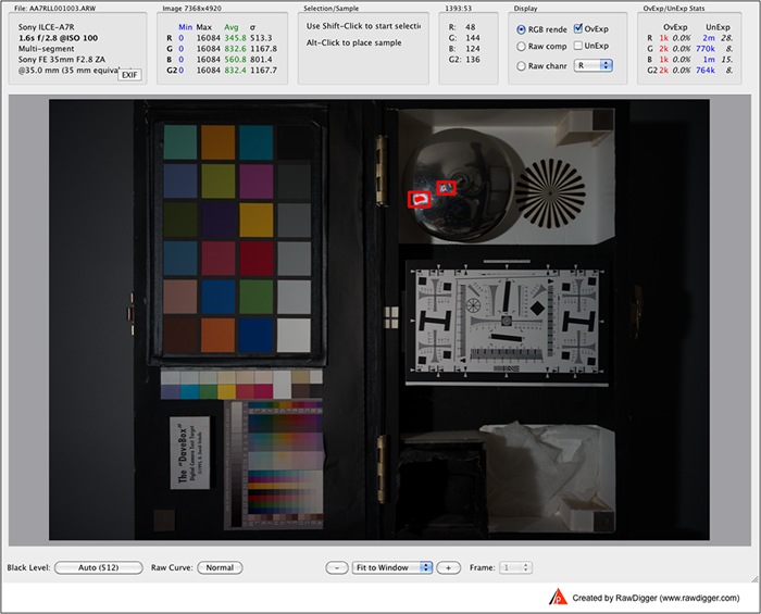
Figure 27. Sony A7R.
On a normally exposed image, you will have at least a few of the overexposed pixels in every major specular highlight (if there are such highlights in the scene, of course). If some highlights that are specular in nature do not have overexposed pixels even if looking at 100% magnification the image should normally be considered as underexposed. As it was already mentioned, curved metal and glass surfaces are the first candidates for these specular highlights, as well as all of the sources of light in the image.
And two final notes to those of you who decided to experiment with your cameras:
- It is easier to recognize and analyze the specular highlights if the area is large enough and placed over a much darker background.
- If you are using a full-frame camera, or a medium format camera, place the specular highlights slightly off-center to avoid the areas of technological stitches to have a better view of the histogram (different parts of the stitched sensor often have different characteristics and the histogram is not so easy to read if those are mixed.)
To see how the sensor is stitched lets take a fully blown out shot:
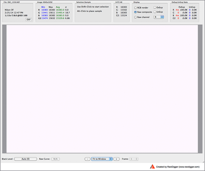
Figure 28. Fully blown out shot
To exaggerate the contrast we use the Per Channel black level settings in Preferences:
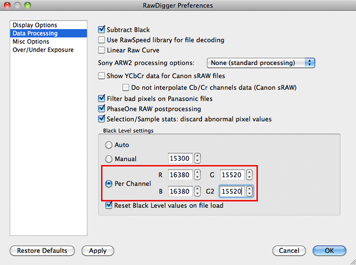
Figure 29. Setting Black Level manually, per channel, in RawDigger Preferences menu
… and inspect the displayed structure:
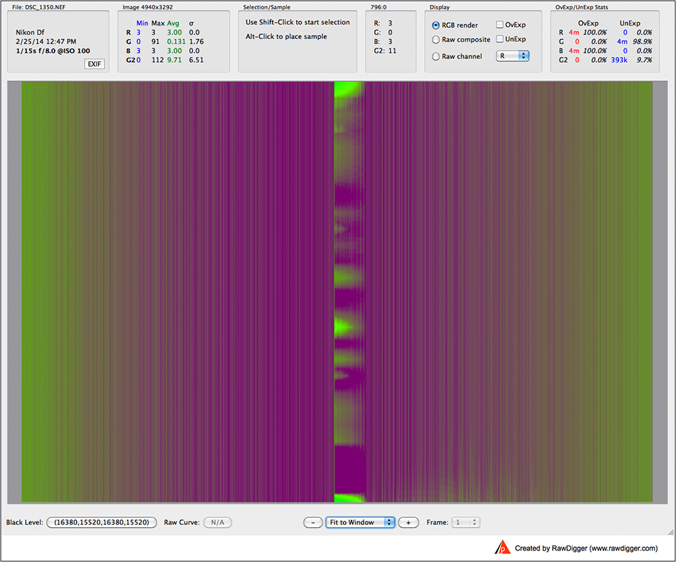
Figure 30. Nikon Df. Sensor stitching structure
Though the difference between the stitched halves is very small it is obvious that the “left” part of the sensor is more uniform and better suitable for analysis.
This article in PDF format: RawDigger_Histogram_Part_III_Overexposure_Shapes.pdf
The Unique Essential Workflow Tool
for Every RAW Shooter
FastRawViewer is a must have; it's all you need for extremely fast and reliable culling, direct presentation, as well as for speeding up of the conversion stage of any amounts of any RAW images of every format.

Now with Grid Mode View, Select/Deselect and Multiple Files operations, Screen Sharpening, Highlight Inspection and more.
5 Comments
Masked pixels
Submitted by Francisco Disil... (not verified) on
Hi, Thanks for the detailed explanation.
I'd like to add to check that you have the "Masked Pixels" option unchecked in the Preferences -> Display options.
Some cameras have reference pixels hard-wired to min an max numeric levels in the masked pixels area, which will show as a spike in the histogram where there should be none. This is easy to note in cameras that have different blown out levels for different channels, such as some Nikon models. In those cases, you will see a spike at blown out level and then another small spike at the maximum numerical value (depends on bit-depth)
Regards
Thank you, Francisco, your "
Submitted by Iliah Borg on
Thank you, Francisco, your ""Masked Pixels" option unchecked' comment is quite important.
--
Best regards,
Iliah Borg
Hi. I'm sorry for asking an
Submitted by John (not verified) on
Hi. I'm sorry for asking an unrelated question here. How is the position of EV0 specified on histograms? Thanks a lot.
By default, we set zero to -3
Submitted by Iliah Borg on
By default, we set zero to -3 EV down from maximum raw value (equivalent to 12.5%), which is very close to the most common standard recommendation (78/Hsat). In Preferences -> Histograms -> "Set histogram EV0 by" drop-down allows to switch between maximum camera data range and maximum for the current frame. The description is in Manual, http://www.rawdigger.com/usermanual/preferences , under "Histograms Tab".
Additionally, the Histogram window offers controls over the histogram range - please have a look at the Manual, "Histogram representation in photographic mode", http://www.rawdigger.com/usermanual/histograms - this is useful for darker shots, when there is not enough data for the Auto to work correctly. So, one can uncheck "Auto" here and set the range.
--
Best regards,
Iliah Borg
Thank you. Really a great
Submitted by John (not verified) on
Thank you. Really a great site with full of great info. I'll try the software soon.
Add new comment