Unlike film sensitivity, which can be measured using a standard procedure, the sensitivity of a digital camera is somewhat a fuzzy concept. In particular, the existing ISO 12232:2006 standard implies the use of the output image in sRGB (see a summary of the method in Wikipedia http://en.wikipedia.org/wiki/Film_sensitivity#Digital_camera_ISO_speed_a...), which, in turn, implies the use of a raw converter (either the in-camera one, or a stand-alone). The fact that a converter can skew the data in various ways like overlaying a tone curve, or adding a hidden exposure adjustment is not accounted for in the ISO standard.

As a result, the sensitivity of the camera turns out to be a pretty random variable (which is noted in the abovementioned Wikipedia article), and the camera manufacturers do not make it easier for the user, adding quirks of their own. For instance, cameras from different manufacturers can be of the same sensitivity nominally, but can behave differently when it comes to the exposure latitude, thus resulting in the user having to adjust and relearn when switching cameras. Furthermore, these quirks can be observed when using different settings on the same camera.  For example, ISO 50 and ISO 100 for the same Canon 5D mark II turn out to be the same sensitivity, which means the same exposure on these two sensitivity settings gives out the same signal, although, one would expect that it should doubly differ.

Further on we will discuss a simple method, which allows us to calibrate the exposure meter in such a way that on different cameras (or on different sensitivity settings of the same camera) the results are predictable.

The characteristics curves of the digital sensor and film

The characteristics curves of standard film and a digital sensor are cardinally different on the edges of the operative range, which is illustrated on the next diagram, graphed based on the coordinates exposure logarithm signal logarithm (for film optical density, i.e. logarithm of transparency):

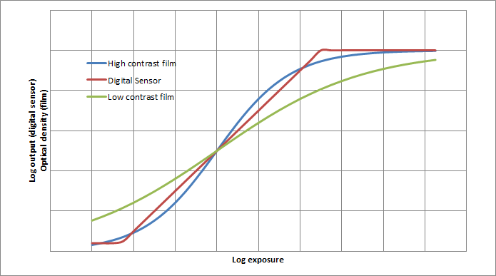
The curves on the diagram are modeling curves, a logistic equation is used for film, and a linear relationship with an instant color saturation is used for digital sensor.

In real life, we deal with 3 (sometimes 4) color channels, the sensitivity of which is not the same (meaning that a grey patch under a specific light will gives us 3 or 4 different responses) and we deal with 3 (or 4) characteristics curves, rather than 1. In the coordinates of the above-mentioned diagram, different sensitivity means the displacement of the characteristics curve horizontally, left or right.

As we can see from the diagram, the behavior of the digital sensor is very different from the way film behaves.

Behavior in highlights

• The characteristics curve of the film is smoothly bending, the details in extreme highlights are reproduced, even if with a low contrast. 
• The sensor enters the saturation mode instantly, the details brighter than a certain threshold become undecipherable. In practice, oversaturation of the sensor s pixels can result in blooming (the bleeding of the signal charge from extremely bright pixels onto the neighboring pixels), which means that not only the oversaturated pixels will be overexposed, but also the neighboring ones will suffer the same fate.

Behavior in halftones

• The digital sensor is linear (the output signal is liner proportional to the cast light), the slope of the characteristics curve (log-log) will remain constant (equal to 1), thus the sensor contrast is constant throughout the entire working range (and for all digital sensors). Exposure of halftones lighter or darker than the exposure meter suggests at a first glance doesn't seem to alter the contrast transfer (in reality, there is a difference, due to a large nonlinearity of the sensor in shadows and a smaller number of reproduced shadow gradations)
• Different films have different contrast coefficient, and the slope of the linear portion of the characteristics curve is different. Exposing halftones so that they do not fall on the central portion of the operative range of the characteristic curve changes the contrast reproduction.

Behavior in shadows

• In shadows, film gradually loses contrast, the bend of the characteristics curve is relatively smooth
• In shadows, the sensor loses gradations: since the coding of the signal is linear, therefore when moving into the shadows area, every subsequent exposure stop (reducing the exposure by 1EV) has half as many different signal levels. Thus, due to the noise, there is also loss of contrast.

With the increase of the sensitivity of the sensor (i.e. increasing the coefficient of signal amplification prior to and/or after digitization), the relative amount of noise also increases, meaning the linearity is broken further. Firstly that affects shadows, secondly halftones, since the sensor behavior in highlights is the least likely to change.

Exposure metering

While measuring the exposure based on the light reflected from the subject, we assume that if we set the exposure based on the reflected light, then this object will show as a midtone on the image.

The calibration constants of exposure meters made by different manufacturers vary, since some manufacturers of exposure meters and cameras (including Canon, Nikon, Sekonic) assume that the medium tone is approximately 3.15 EV lower than the highlights. The second group of manufacturers (Pentax, Minolta, Kenko) assumes that the medium tone is approximately 0.4 eV lighter. You can read further about the exposure meter calibration constants on Wikipedia http://en.wikipedia.org/wiki/Light_meter#Calibration_constants.

While printing, the midtone is usually represented as 18% grey (if you count in stops, then that is 2.47 EV lower than 100% white), thus the first group of photo equipment manufacturers imply the compression of approximately 0.7 EV of the range from the midtones to highlights, while the second imply the compression of about 0.3 EV.

Of course, in the real world, all scenes are different; therefore a film photographer has to simply understand where in the midtones range the subject falls (if exposed in accordance with exposure meter ) given that all the other procedure steps (film, developing, printing) are standard and accomplished within permissible tolerance. Still, the bright highlights will be compressed, the highlights contrast will decrease, but some detailing will remain. The abovementioned is relevant firstly to negative film, slides behave less tolerably, but the characteristic curve also smoothly bends in highlights and in the shadows.

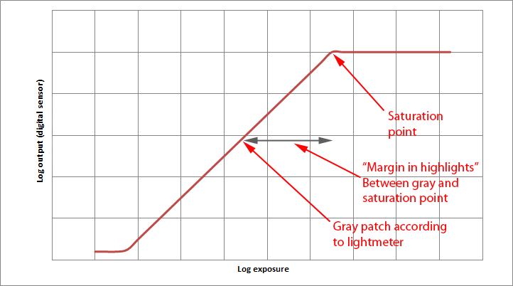
In the case of a digital sensor, there is no compression of highlights, and the saturation happens abruptly. All details brighter than the saturation point will not be reproduced. As a result, while shooting with a digital camera, one has to know the difference between the saturation point and the measuring point of the exposure meter.

Measurement method

The suggested exposure meter calibration method consists of shooting an image of a grey step wedge using two exposures:

1. In accordance with the exposure meter, to obtain the calibration point of the exposure meter on a given camera
2. With a very large overexposure (5-6-7 stops), to obtain the sensor saturation level for the given camera.

Next we use the averaged values of the pixels (from the raw file) for both exposures, divide them, getting the headroom in highlights as a factor, finally, taking a log base 2 we are getting the result in measured in photographic stops, EV.

There are, however some complications.

1. The relative (relative to each other) sensitivity of the channels is different under the lights of different spectrums. As a result
   • Under a given lighting, the headroom in highlights will be different for different color channels
   • With a change in lighting, the headroom in highlights also changes
2. After changing the sensitivity setting on the camera, the headroom in highlights can also change:
   • The saturation level can change, while the values obtained while shooting according to an exposure meter remain the same
   • The set ISO can be artificial, and the exposure meter is not aware of that.

The spectral sensitivity of the exposure meter can differ from the spectral sensitivity of the sensor.

As a result, it is best to calibrate the exposure meter on every sensitivity value that is used, and under every lighting source used.

Testing

In the following tests we used an Olympus E-PL3

Lets shoot two abovementioned images:

1. the grey target (a grey patch can also be used, as well as plain white paper, without optical whiteners). Turn off all exposure adjustments and shoot. If the target takes up the entire field of view of the shot, then the setting of the exposure meter does not matter; all settings (spot, matrix, center-weighted) will result in the same exposure. To obtain even brightness in the shot, it is best to use long lens, slightly (1-2 stops) stopping down the aperture. It is useful to slightly de-focus the lens, to make sure the inevitable irregularities and dust on the target are not an issue.
2. The same shot, but with an exposure adjustment of +5..+6 stops (EV). A smaller adjustment works fine on many cameras, but you can t overdo it.

Load these shots, one by one, into RawDigger, make a Selection in the center of the shot and observe.

Daylight

Saturated image

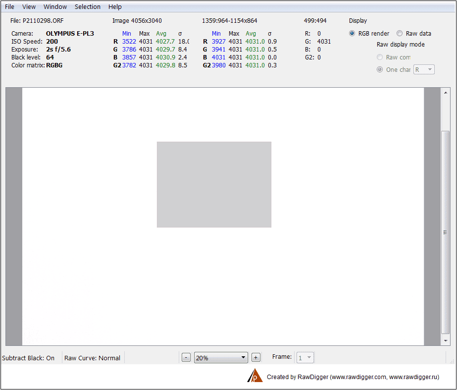
As we can see, the signal of the given camera, despite the saturation, varies between 3522 and 4031 along the entire shot (informational block Image ) and between 3927 and 4031 along the selected area (the next informational block). But the middle sample value in the central part of the shot is 4031 in all channels, which corresponds with the maximum. Therefore, there are very few pixels deviating from the maximum, which is very apparent on the histogram of the sample, in the linear scale the only visible value along the vertical axis is 4031:

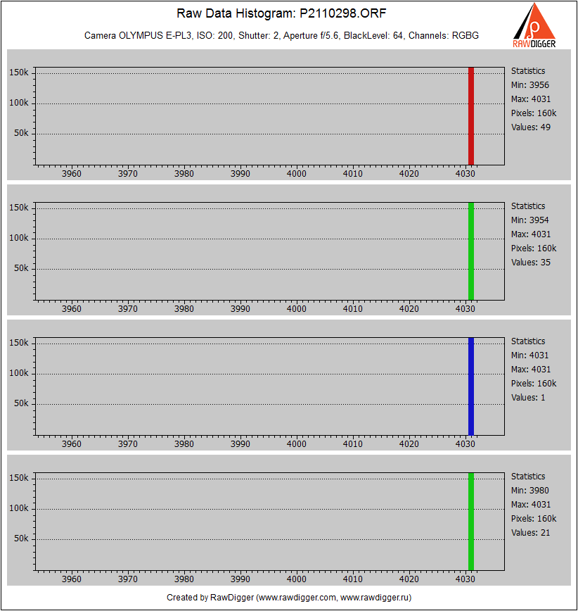
Only in the log scale other values are visible, although there are very few of them a couple of dozens of each, whereas the main value is seen around 160 thousand times in each channel.

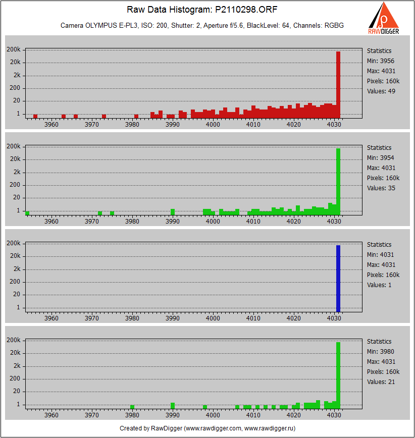
Therefore we know the saturation value: 4031 for each of the color channels.

Image with the exposure according to the exposure meter

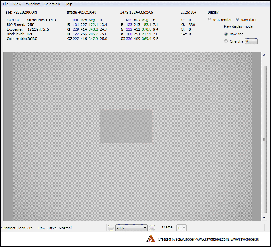
It is clear that the optics vignettes slightly, so lets take the area in the center of the image, and the medium values on the channels. In the given example, it is 183 (R), 370 (G), 218 (B), (the third informational block above the window, counting from left to right, Avg column). We ll disregard the difference of 0.5 between the two green channels.

Divide the maximum possible values (from the overexposed shot) by the channel values of the grey patch according to the exposure meter, and we get the headroom in highlights .

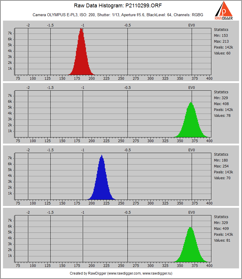
The per-channel difference is visible on the histogram of the sample. The 0 EV value on a photographic scale is set to 370 (the average of the green channel on the sample), the relative underexposure of the blue (.8 EV) and the red (1 EV) channels is clearly visible.

Artificial lighting

When lighting with an artificial source of light, the result changes: the image of the grey target has less blues and more reds, which is not surprising, since the grey card is neutral, and the light spectrum has changed (moved to the reds), and the color filters in the pixels remained the same. The headroom in highlights in the green channel also increased a little.

Here is a histogram:

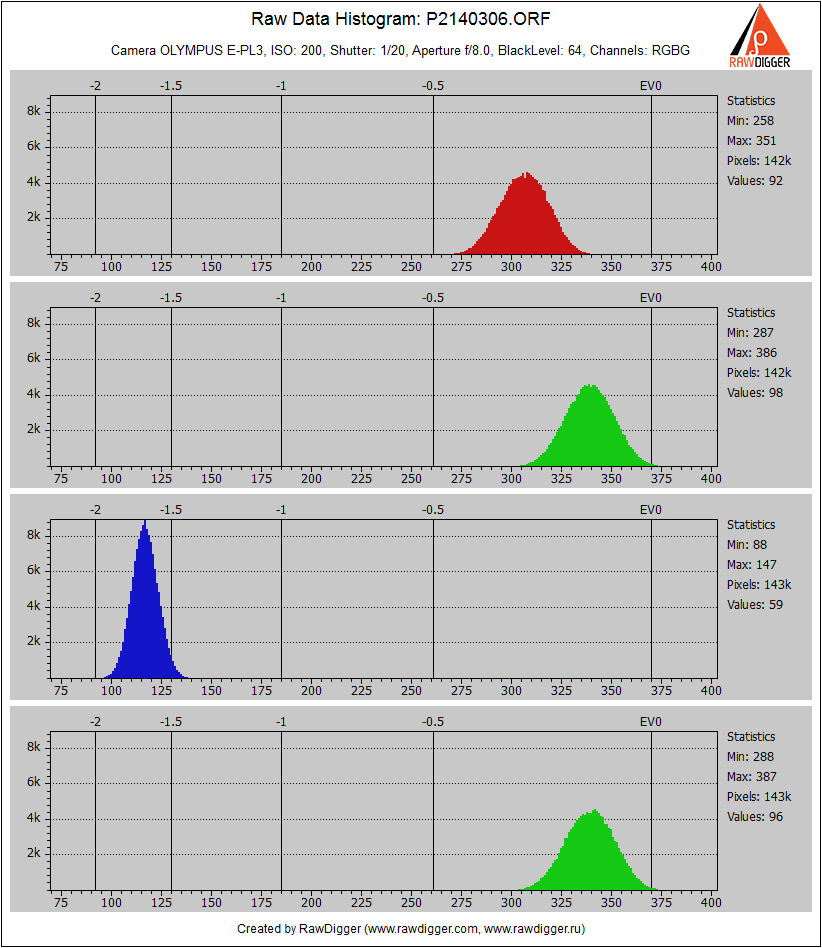
This histogram is made with the same horizontal axis scale as the last one. It is obvious that the channel imbalance is cardinally different: the blue is undersaturated by 1.5 EV relative to the green, and the red is exposed practically the same as green.

How to use this

The knowledge of half of the photographic latitude (i.e. headroom in highlights , the difference in brightness between the halftones of the image and the brightest subject which is still visible) allows to confidently assess the exposure

Exposure for highlights

In the case when the scene has a large range of brightness, but it is known what highlights have to be fully detailed, the exposure assessment is trivial

1. Do a test measurement of the highlights (with the in-camera exposure meter in spot mode, or a hand-held exposure meter)
2. Adjust the exposure slightly less than the headroom in highlights (+ 3..3.3 EV for the camera in hand and daylight)

This is basically it. The necessary highlights will be preserved and well-defined in full detail, which is what we were trying to accomplish. This method is especially useful if the light parts of the shot need to be fully developed, but still light, for instance while shooting a winter scene.

Exposure for midtones, with monitoring the brightness range of the scene

Lets assume that the midtones define the exposure of the shot, and we do not want to change it.

Determine the exposure for midtones and once again use the spotmeter (or the camera exposure meter in spot mode) to determine the highlights exposure, since if it differs with the desired one by a value larger than the headroom in highlights then the highlights will be blown out. Therefore, we have to either somehow decrease the contrast of the scene (gradient filters, or lighting of the foreground) or we have to change (decrease) the exposure, or look for a different angle, so we don t have the interfering bright highlights.

Controlled overexposure

If the bothersome highlights have a near-neutral shade, and the raw converter we are using is capable of Highlight recovery, than you can risk it and leave the details in only one or two channels out of the three. If we set the exposure to a bit higher than is allowed by the headroom in highlights in all three channels, then we will lose details in the most sensitive channel (usually green), and can then recover something similar to details using other, non-clipped channels.

For the given camera and daylight, this allows for an extra 1 EV to the headroom in highlights.

What about the camera histogram?

A thoughtful reader will ask us why do we need all these tricks if there is a camera histogram.

Yes there is a camera histogram. But let s recall during our testing we shot a grey card. Therefore on the in-camera histogram, given a correctly set white balance, we will see peaks in the same places for all the color channels (because the card is grey, and the white balance is correct, it can even be set based on the card).

But do these peaks accurately illustrate what happens in real life? For the daylight, we have 1 stop undersaturation of the blue and red channels (relative to the green), and the camera places the peaks in the same location. Under artificial lighting, there is a 2 stop blue undersaturation, but the camera will show its peak in the same place as the red and green.

The same thing applies to the oversaturation indications. You can somewhat trust it only for the green channel, but you cannot really tell what happens with the other channels based on the camera histogram and the standard white balance presets.

Of course there is UniWB, but its usage in many cameras is complicated by the fact that the camera doesn't save the data about the natural white balance at the time the shot is taken, which complicates the post processing of images. Besides that, UniWB does not solve the task entirely, since besides the white balance, the camera applies some unknown tonal curve, and what will be cut off as a result of that, and what will remain is unpredictable.

The camera histogram is especially bad under artificial lighting, the channel imbalance reaches about 2 stops or more, meaning that the blue channel overexposure indicator will most definitely lie, making the photographer decrease the exposure and cause even higher underexposure in the blue channel.

Also the knowledge of headroom in highlights for your own camera for different settings allows one to control the shooting without the camera screen. The results are guaranteed without it.

The Unique Essential Workflow Tool

for Every RAW Shooter

FastRawViewer is a must have; it's all you need for extremely fast and reliable culling, direct presentation, as well as for speeding up of the conversion stage of any amounts of any RAW images of every format.

Now with Grid Mode View, Select/Deselect and Multiple Files operations, Screen Sharpening, Highlight Inspection and more.