
Submitted by lexa on
Unlike its film-using predecessors, modern digital cameras present us with a challenge of a non-replaceable sensor. Due to this, the given amount of light, which falls on an element of the sensor (pixel), creates the same charge irrespective of ISO sensitivity setting resulting in an identical output signal. The response of the sensor itself depends only on the light, and not on the digital camera sensitivity (ISO) setting.
It would seem that this contradicts everyday photographic practices: if there is not much light, you have to set the sensitivity (ISO value) higher, and the picture will come out right, but if you set the sensitivity low, then it won t come out right. Lets have a closer look.
Basic Concepts
The camera sensor is a sort of photon counter. It transforms light hitting each pixel of the sensor (photon flux) into electrons. The amount of electrons created in the pixel is proportional to the amount of photons captured. This coefficient of the proportionality is called Quantum Efficiency (QE). QE is a characteristic of sensor design; it does not change when you alter the camera s settings (changing sensitivity or the like). As a result, the same amount of photons that land on one particular pixel creates approximately (taking into consideration that the process is probabilistic) the same amount of electrons inside it, independent of the camera settings.
Pixel Charge Capacity: every single pixel can be characterized by the fixed maximum number of electrons it can hold. Often this capacity is referred to as Full Well Capacity (FWC). If the quantity of electrons produced during exposure exceeds that number, the extra electrons will either flow into the neighboring pixels (the well will overflow and there will be a blooming effect, that is the neighboring pixels will be pseudo-exposed due to the charge spill from the overwhelmed pixel), or those excessive electrons will be drained through the anti-blooming sensor schematics. Obviously, if there is less light hitting the sensor, there will be fewer electrons produced. Pixel capacity of a particular sensor depends on the area of the pixel, and, as it seems, on the sensor electronics design, as well as on other factors (mainly temperature). Typical values for modern dSLRs are several tens of thousands of electrons per pixel. It is obvious, that the capacities of different pixels forming the same sensor are slightly different because of manufacturing intolerances. This difference we will disregard in the following discourse.
Value read-out: after the exposure, an analog read-out of the pixel charge (number of electrons produced during the exposure) occurs, and the ADC (analog-to-digital converter) converts the charge value into digital form. Typical ADCs used today are capable of 12-14 bit conversions, meaning the range of the output values is 0 4095-16383
Consequences of Basic Concepts
True sensor sensitivity (and lowest camera real ISO sensitivity setting) is determined by the capacity of the well. The amount of the light that hits the pixel must be such that the well does not overflow. If the amount of electrons formed exceeds pixel capacity than we will not be able to differentiate the amounts of light in the two different pixels they are both overflown, and will give the same result during the read-out. Taking into account that the typical capacity of a pixel (in electrons) is greater than the maximum value of a typical ADC (in AD units, ADUs, sometimes also called "DN" for Data Numbers), on minimal sensitivity several electrons read from the pixel create one ADU at the output (in raw data), that is the conversion factor is less than 1.
With the reduction of falling light (due to lowering the brightness of the scene or reducing the exposure) the amount of electrons produced in the pixels of the sensors is also reduced. If one preserves the camera settings for minimal sensitivity, the conversion factor electrons/signal remains the same, and if there are fewer electrons then obviously the output signal (values in raw file) will become smaller.
If one changes the sensitivity (ISO) value of the camera, the coefficient of the amplification (gain), or/and the input range of the ADC will change. In this case, the ratio of electrons/signal will reduce, while the signal (raw value) will grow (for the same amount of electrons formed on the pixel).
Unity gain at some value of the camera sensitivity it happens that 1 electron produced in a pixel results in 1 ADU at the ADC output, that is the conversion factor is now equal to "1".
Because a pixel contains an integer number of electrons, raising the sensitivity setting any further has very little sense. In fact, if, in some pixel, we have 10 electrons, and in another pixel we have 11 electrons, no amount of amplification is going to help us achieve real intermediary levels. True, that with an amplification factor of 10 (for instance) times, due to noise we can achieve 101 from the first pixel and 109 from the second one, but this will be noise and nothing but noise we will not gain anything by way of real tonal gradation.
There is certain sense in increasing the amplification:
- To drive the the signal higher than the level of noise of the ADC (helps if the noise of the amplifier is significantly lower than the noise of the ADC, which is the result of an unbalanced design).
- To drive the signal higher than the level of the dark current, which allows us to reduce the non-linearity in the shadows, especially if the subtraction of the black is done in the camera and using integer math.
- The translation of the signal (raw value) into a zone that is comfortable for raw converter (some converters being set at defaults clip input data in highlights and plug shadows).
But, in general, the gain from amplification higher than unity would be relatively small.
As a result, the unity gain mode is especially favored by astrophotographers (and other photographers, shooting low light scenes), because it gives the greatest balance between necessary shutter speed and noise on the photograph.
A question emerges: how to determine that magical sensitivity setting on your camera? This is where photon noise comes in.
Photon Noise
Photon noise is a property of any natural (maybe a bit different with lasers) flux of light: the flux is not constant; the amount of photons constituting it over time follows Poisson distribution; meaning the square of the standard deviation (StdDev) of a signal (σ2) is equal to the mean value of the signal itself, and hence the StdDev (σ) is equal the square root of the mean value of the signal.
Thus, we must photograph a smooth patch of a card (or, at least, a smooth surface area), and find such a sensitivity, where the square of StdDev is equal to the mean of the signal itself.
In practice one should take a white (the brightest) patch, setting the exposure in such a way so that there would be no clipping of the maximum values. In this case the contribution of other noise sources (noise from digitizing, thermal noise, etc.) will be as small as possible. The correct procedure (which is used by astrophotographers) includes an evaluation of non-photonic noise sources, so as to isolate precisely the photonic part. In practice the contribution of these sources to the noise of the signal recorded for the white patch on the average values of sensitivity is not great, but it is there, so we will be satisfied with such ISO setting, where the square of StdDev is so slightly higher than the signal.
Now for Practice: Canon 5D Mark II
We will be using a readily available archive of examples from the site imaging-resource.com to take from there those test images which contain a smooth, white patch. For example, this one:
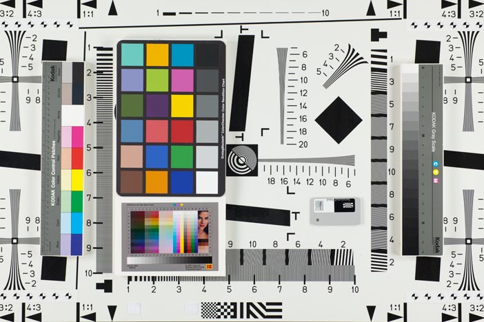
Picture 1.
These images contain the white patch on X-Rite/Macbeth ColorChecker CC24 (to the left of the center) and a similar patch on the Kodak Q13 Color Control Patches strip. Any of those is suitable for our purposes.
Raw files containing the shots of this scene for different ISO sensitivity values can be downloaded from http://www.imaging-resource.com/PRODS/E5D2/E5D2THMB.HTM
Open one of the files in RawDigger and select the white patch (marked as 1 on the illustration below). The statistics for the selection will be presented in the Selection/Sample portion of the Info view (marked as 2 ); the metadata from EXIF is displayed in the leftmost area, marked as 3 . Metadata includes file name, camera make and model, ISO sensitivity setting, shutter speed and aperture value.
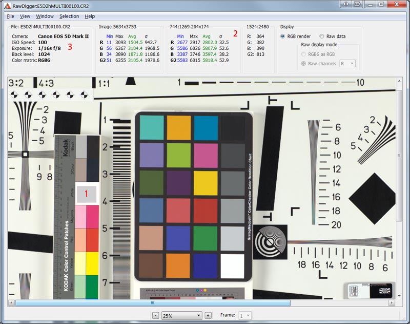
Picture 2.
Without removing the selection, we will sequentially open photos taken with different ISO sensitivity settings while looking at the mean (Avg) value and the standard deviation ( ) in the green channel. The results we will record in a table like the one below (the data in the 4th column is the square of the standard deviation which occupies the 3rd column): the necessary condition of the square of StdDev is slightly higher than the mean of the signal is achieved at the ISO 400 (in bold in the table).
| Shutter Speed and Aperture | ISO | G channel average |
σ | σ2 |
| 1/8s f/8 | 50 | 11833 | 89.6 | 7885 |
| 1/16s f/8 | 100 | 5808 | 52.5 | 2756 |
| 1/25s f/8 | 200 | 6369 | 67.8 | 4596 |
| 1/64s f/8 | 400 | 5918 | 85.1 | 7242 |
| 1/128s f/8 | 800 | 5840 | 111.8 | 12499 |
| 1/256s f/8 | 1600 | 5683 | 150.6 | 22680 |
The shot for ISO 200 is somewhat knocked out of the common order, the value of the green channel being ~6400, instead of ~5900 like it is on the other shots (except ISO 50 shot which we will discuss a little later). This happened because the combination of shutter speed and aperture value in this shot is also knocked out of the linear progression, by virtue of unknown cause the shot is taken on 1/25s f/8 , whereas in linear progression 1/32s f/8 should have been used.
Despite this the data even in the green channel is not clipped: maximum values on the shot is 6367 (informational block Image , second from the left), while in our selection it is only 6026. The same can be seen on the histogram (to see the histogram, use Menu - Selection - Selection Histogram):
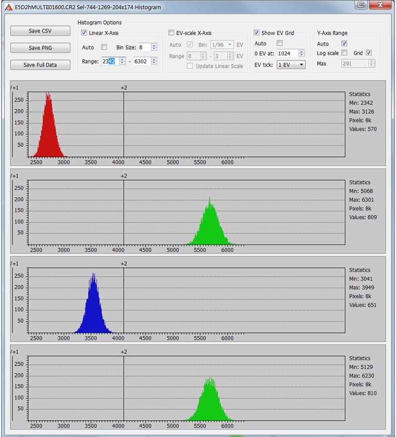
Picture 3.
The histogram above is for ISO 1600, for smaller ISO values peaks are narrower (the variance is less), and clipping is also absent.
ISO 50
On the given camera ISO 50 is actually nothing else but ISO 100 with exposure correction of +1 EV. While looking at the table with different sensitivities (first table in the text), it can be observed that the shot at ISO 50 setting is taken with the twice the exposure of the ISO 100 shot, and the signal level is practically twice as large (a bit less than twice as large, but within the allowances on the accuracy of the shutter).
Thus we can determine that the coefficient of the amplification for the ISO 50 setting is the same as for the ISO 100, meaning it is the same sensitivity .
Pixel Charge Capacity (Full Well Capacity, FWC)
The coefficient of amplification (or gain) on the lowest true setting of sensitivity (ISO 100) is 4 times lower than for ISO 400. For the ISO 400 the coefficient of amplification is about equal to one. Accordingly, for sensitivity of ISO 100 this coefficient is equal to 0.25. Maximum value at the output of the ADC is about 14000, and we can conclude the pixel capacity is no less than 56000 electrons.
Real FWC may be a bit larger as the range may be artificially limited, but the data we got in our measurement is not enough to substantiate such deduction.
Practical Findings
- Raising the sensitivity beyond ISO 400 on this camera should be done only in extreme circumstances, for example, if the raw converter of your choice renders shadows particularly poor. One should expect a substantial gain in image quality compared to underexposure (and subsequent push-processing in a good raw converter) only if the pre-ADC amplification pushes the signal level from the sensor higher than the level of ADC noise.
- ISO 50 is the same thing as ISO 100 with an overexposure of 1 stop. There is no point in this ISO setting.
The Unique Essential Workflow Tool
for Every RAW Shooter
FastRawViewer is a must have; it's all you need for extremely fast and reliable culling, direct presentation, as well as for speeding up of the conversion stage of any amounts of any RAW images of every format.

Now with Grid Mode View, Select/Deselect and Multiple Files operations, Screen Sharpening, Highlight Inspection and more.
17 Comments
Unity gain
Submitted by Kaa (not verified) on
So, you believe the unity gain ISO for 5D2 is 400? That's an unusual claim. Typically the unity gain for 5D2 is considered to be ISO 1600 (see e.g. http://www.clarkvision.com/articles/digital.sensor.performance.summary/#...).
Roger Clark's numbers are for
Submitted by lexa on
Roger Clark's numbers are for '12-bit unity gain' (kind of common denominator for all cameras). But 5D2 is 14-bit camera. Yes, for (imaginary) '12-bit output' the unity gain will at 1600ISO
Ah, yes, you're correct.
Submitted by Kaa (not verified) on
Ah, yes, you're correct.
small correction
Submitted by adj (not verified) on
Thank you for this excellent application, and informative article!
I noticed a small typo:
"We will be using a readily available archive of examples from the site imaging-resources.com"
That should be imaging-resource.com without an 's'
Thanks! Corrected.
Submitted by lexa on
Thanks!
Corrected.
Has anyone calculated this for Pentax K-3 II std vs PSR ?
Submitted by Darren Addy (not verified) on
This is a VERY good article and is logically presented. I am very interested (especially from an astrophotography perspective) what the Unity Gain ISO is for the Pentax K-3 II (and also) for the Pentax K-3 II RAW file produced by the Pixel Shift Resolution (which reads out the sensor 4 times, shifting the sensor by 1 pixel between read outs - eliminating the need for de-Bayering). This is a revolutionary concept and has implications for astrophotography (albeit only at a maximum exposure of 30 seconds, the camera's shutter speed limit for using PSR). Due to this innovation, it would be interesting to seeing a 2015 revisiting of this subject, particularly comparing at the Pentax K-3 II and its Pixel Shift Resolution. (This camera also has no AA filter, which is not addressed AT ALL as being a factor in the accuracy of the pixelsites' recording of photons.)
Pentax K3-II stores four
Submitted by lexa on
Pentax K3-II stores four images (one for each exposure) in RAW file.
So, from pixel capacity/amplifier gain side nothing changed.
Why is Std Dev less than SQRT(mean) at medium-high exposure?
Submitted by Ted Cousins (not verified) on
I shot the MacBeth mini-card under CFL lighting with a Sigma SD1M:
http://kronometric.org/phot/temp/SDIM0392.X3F
Here are the 6 results for the neutral patches:
http://kronometric.org/phot/temp/RAW%20vs%20lux%202.gif
I can understand that the measured SD could be more than SQRT(mean) but I don't understand how it could be less.
Please help,
Ted
For example, if amplification
Submitted by lexa on
For example, if amplification is less than 1e->1ADU (so some kind of averaging in ADC), than SD will be less than SQRT(mean).
amplification versus SD < SQRT(mean)
Submitted by Ted Cousins (not verified) on
Thanks, Axel,
I'll have to research the e- per ADU.
The SD1M blue channel also had missing levels in the histogram, because of Sigma's stupid in-camera 10-bit look-up table (not sure of purpose) applied before writing to the card.
I'm surprised the SD1M takes any pictures at all ;-)
Ted
Histogram for small selection
Submitted by lexa on
Histogram for small selection in 3rd gray patch: https://www.dropbox.com/s/poulyqj4cqg8ilh/Screenshot%202016-01-16%2023.3...
It looks like Blue channel is processed in some way (missing values), while R/G are not
Conversion Factor - which way up?
Submitted by Ted Cousins (not verified) on
In file:///C:/Users/Ted/Desktop/SNR%20SD1%20HI%20card/Determining%20pixel%20charge%20capacity%20and%20amplification%20gains%20for%20a%20digital%20camera%20_%20RawDigger.htm it says:
"Taking into account that the typical capacity of a pixel (in electrons) is greater than the maximum value of a typical ADC (in AD units, ADUs, sometimes also called "DN" for Data Numbers), on minimal sensitivity several electrons read from the pixel create one ADU at the output (in raw data), that is the conversion factor is less than 1."
This implies that the 'the conversion factor' is ADU/e-
"With the reduction of falling light (due to lowering the brightness of the scene or reducing the exposure) the amount of electrons produced in the pixels of the sensors is also reduced. If one preserves the camera settings for minimal sensitivity, the conversion factor electrons/signal remains the same,"
But that states that 'the conversion factor' is e-/ADU.
Which definition of 'conversion factor' is correct?
Thanks,
Ted
When the conversion is
Submitted by Iliah Borg on
When the conversion is electrons to data numbers, the factor is actually a divisor, so it is less than 1. When the conversion is electrons to signal (volts), it can be, general case, both ways.
The conversion factor remains constant if the settings are the same, regardless of the recording method.
--
Best regards,
Iliah Borg
I'll try a different question . .
Submitted by Ted Cousins (not verified) on
When Axel said:
"For example, if amplification is less than 1e->1ADU (so some kind of averaging in ADC), than SD will be less than SQRT(mean)."
Did "1e->ADU" mean 1e- per ADU or did it mean 1 ADU per e- ?
sorry to be a pain,
Ted
If more than 1 photo-electron
Submitted by lexa on
If more than 1 photo-electron is converted to single ADU unit, than dispersion (σ2) will be less than signal (signal is in ADU units). So, standard deviation will be less than SQRT(mean).
Now I understand :-)
Submitted by Ted Cousins (not verified) on
Thanks Axel.
Blue Channel Processing - Sigma SD1M
Submitted by Ted Cousins (not verified) on
Yes - the SD1M processes channels unequally and the lighting was a simple compact fluorescent.
I should have realized that for a classic photon noise SD it would be nice to have a proper-looking histogram as opposed to Sigma's :)
Thanks for your help, Alex!
Add new comment