Now we are going to illustrate the different histogram display modes. It is often easier to start with some ideal object and than switch to real-world examples. Our ideal object will be a digital simulation of Kodak Q13 Gray Scale. We created a 16-bit 4-channel (RGBG) Bayer-type DNG file based on the Kodak specifications for this scale.

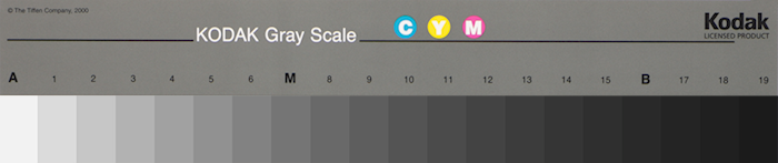
Figure 10.

For this DNG file we’ve chosen the patch size of 32 x 70 pixels, that is, for every one of 20 gray levels represented on Q13 there are exactly 2240 pixels with this level’s value. On a side note, the “A” patch is the white base (bright white paper), “M” is what is considered midtone (close to 18% grey), and “B” is the darkest black that can still hold some details on print.

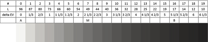
Figure 11. Synthetic Q13 Kodak Gray Scale

… open this .dng file in RawDigger:

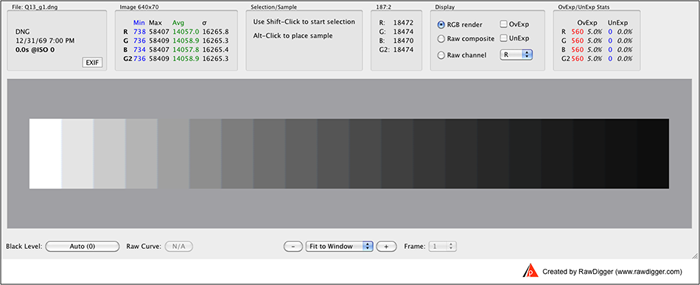
Figure 12. Synthetic Q13 opened in RawDigger

… and look at the histogram of this file:

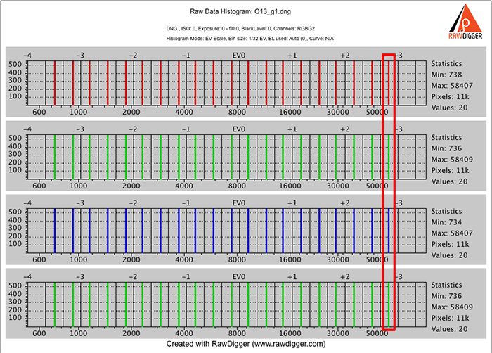
Figure 13. Synthetic Q13 4-channel histogram (RawDigger screenshot)

As you can see on the Fig.10 above, Q13 contains 20 different patches that correspond to 20 different tone values. On the histogram we also see exactly 20 bars for each color channel; each vertical set of four bars (we marked one such set with a narrow red rectangle) corresponds to one patch of the Q13 Scale.

The DNG file was created in RGBG yet we can see that the resulting EV step is indeed 1/3. We see that all bars are positioned per the step prescribed by Kodak and have the same height equal to 560:

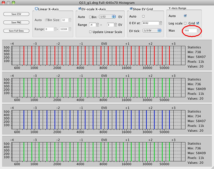
Figure 14.

560 multiplied by 4 (four color channels) gives us exactly 2240 pixels – the total number of pixels in each patch (remember we made the patches of 32*70 = 2240 pixels). This demonstrates how the histogram is calculated: we have exactly 560 pixels in each of four channels assuming each of 20 values existing in the DNG (RAW) file.

When we are dealing with synthetic files – without flare, light un-evenness, vignetting, scratching, you-name-it real life small problems, the histogram is easy to read (and check).

Let’s have a look at a real shot of Kodak Q13 Gray Scale:

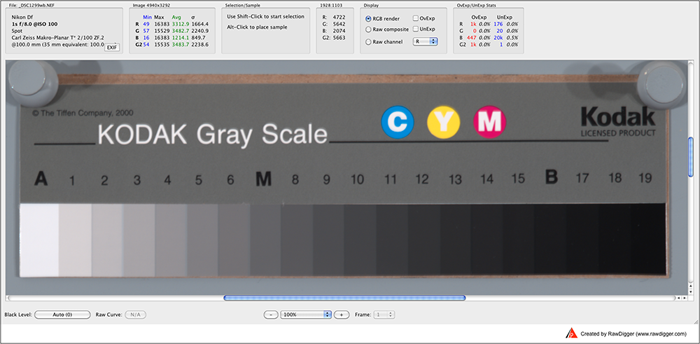
Figure 15.

Now we create a selection (Shift-Click and Drag), which includes all 20 rectangular patches:

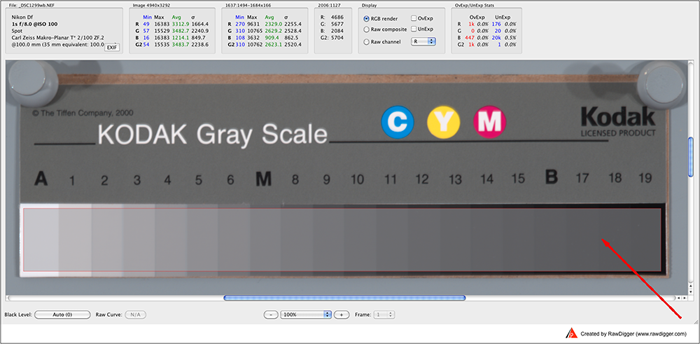
Figure 16. Arrow points inside the selected rectangular area (grey overlay).

And now lets see the histogram of the selected area (right click inside the selected area and choose Show/Hide Histogram)

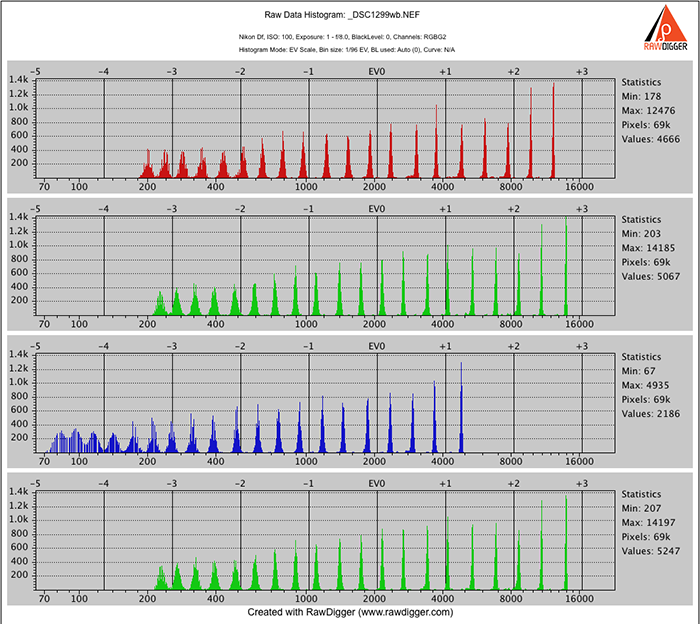
Figure 17.

Instead of 20 sets of 1-level width bars, we see 20 sets of bell-shaped structures of varying widths – from narrow spikes in highlights to bell-shaped curves in shadows. As we are dealing with the real objects here, it is only natural that:

1. The patches on the real Q13 step wedge are not perfectly uniform and evenly spread (manufacturing tolerances, scratches, dust, fingerprints, etc.)
2. The noise (shot noise, a.k.a. photon noise) makes lighter patches wider
3. Flare, glare, and read noise make darker patches wider
4. And, last but not least, pixels on the sensor are not absolutely identical

That is why we see some distribution around the theoretical level value and some deviations. It is common to consider 1/12 EV to be enough precision for photographic light measurements.

As we already mentioned, the design of the Kodak Q13 gray step wedge we are analyzing is such that there is close to 1/3 EV between the patches, and the first step is supposed to be approximately 1/6 EV below saturation maximum. So if both the manufacturing of the target and the reproduction would be perfect (no flare, no light un-evenness, no vignetting, no surface defects, but we are accounting for photon noise) we would have exactly 3 narrow spikes per stop. Aligning the 0 EV so as to have the center of the first spike (more on how to align 0 EV to fixed level see below, Fig.25) at -1/6 EV from maximum, we can see that there are more than 3 bells shapes in the last stop, which most often indicates that the linearity here is less than perfect due to the in-camera flare.

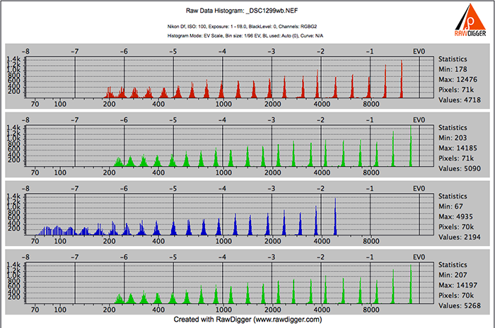
Figure 18.

RawDigger histogram controls and features

Let’s take a closer look at the RawDigger histogram controls and features.

The lower horizontal axis is Linear X-axis, showing pixels values (levels) – on a linear scale.

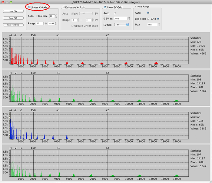
Figure 19. Linear X-Axis

We can check Auto, which mean that bin size will be calculated automatically so that all raw data values – from minimum to maximum - are displayed on the histogram and the histogram fits the window.

We can have a closer look at some values' interval. We just uncheck Auto and manually enter Range limits. Below the chosen limits are from 200 to 4300.

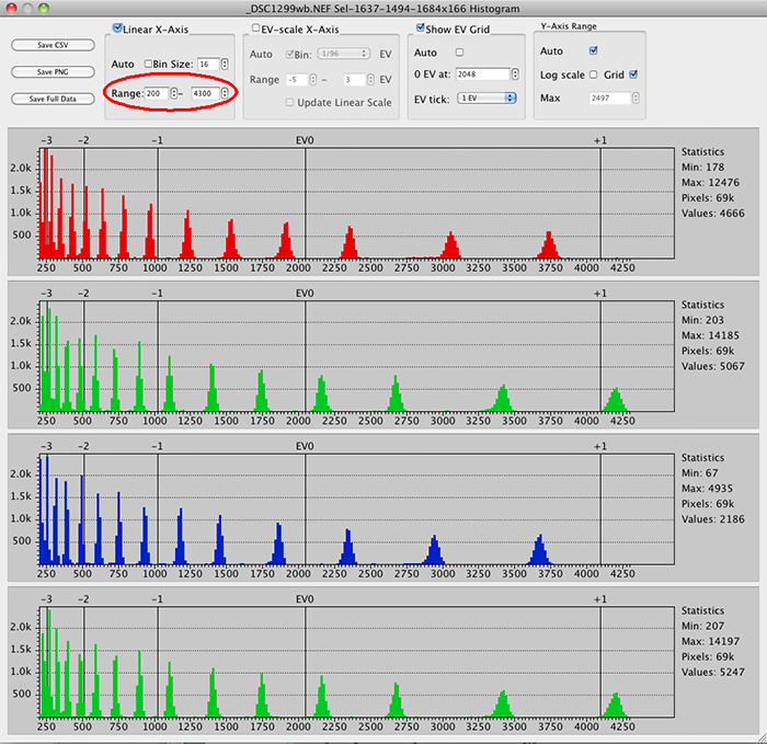
Figure 20. Range from 200 to 4300

We also can change bin size, which gives us a closer look at the values’ distribution:

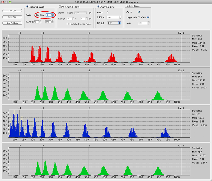
Figure 21. Bin size is changed.

The upper horizontal line represents the X-axis in EV values – EV-scale X-Axis. This EV-scale is logarithmic (log₂ (Linear-X-Axis)).

We usually check the EV-scale X axis together with the next check box Show EV-Grid (if we don’t want to see numbers here, we just uncheck it):

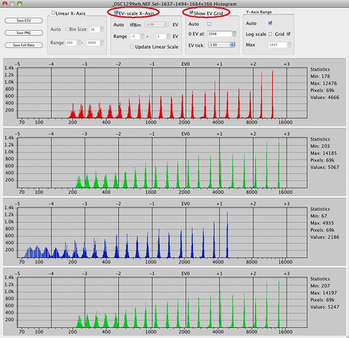
Figure 22. EV-Scale + show EV-Grid

For EV grid we can choose EV tick – to control the grid:

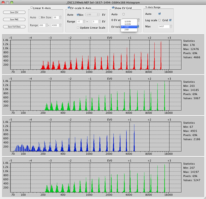
Figure 23. Choose EV-tick

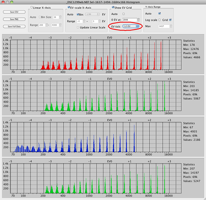
Figure 24. EV tick at 1/3EV

Also, we can choose the position of the zero point 0EV on this axis – 0 EV at:.

For example, we can place it at max value for the Green channel. This will be the “A” patch. 2 1/3 EV lower (see Fig.1) is the “M” patch (the midtone of the step wedge, roughly equivalent to the proverbial 18% grey)

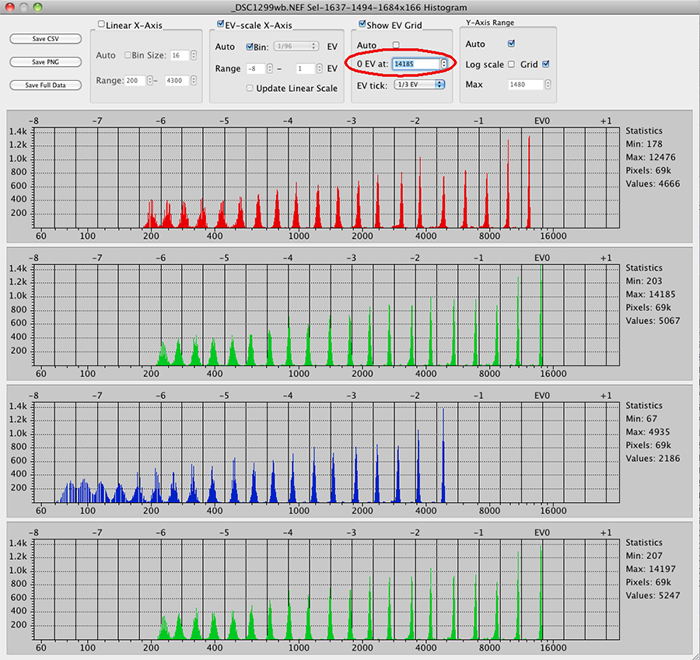
Figure 25. 0EV = max in the Green channel

Y-Axis shows us how many pixels with levels corresponding to X-axis values are found in the raw data of the image.

If “Auto” under Y-Axis Range is checked the scale division value will be determined automatically:

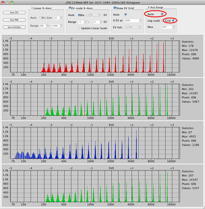
Figure 26. Y-axis, Auto grid size

We can uncheck the Grid box – in this case, the dotted horizontal lines just disappear:

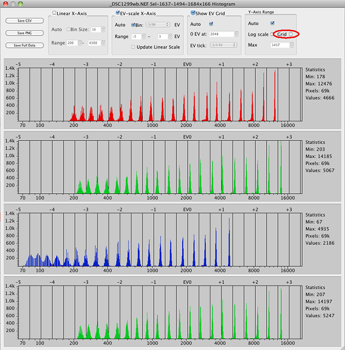
Figure 27.

Also we can choose to use a logarithmic Y-axis - Log scale (if the counts for certain values are so small that the resulting bars are too short to be analyzed, or sometimes even to be visible). Log scale on Y allows to see the bars which go below the radar if the linear scale is in use. This is essential for determining underexposure on the shots that contain specular highlights and relatively small light sources.

Taking a different portion of the same shot that contains the specular highlights we can see how it works:

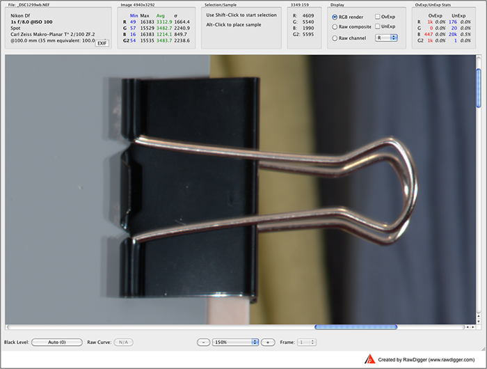
Figure 28.

Let's make a selection (gray overlay inside the red rectangle):

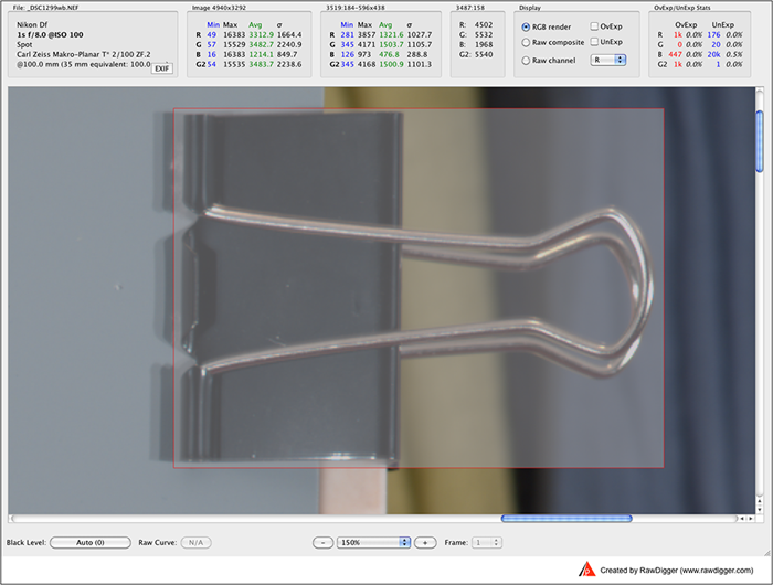
Figure 29.

… and open the histogram of the selection…

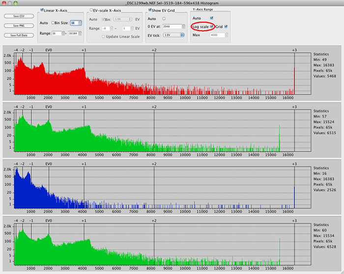
Figure 30. Y–Axis Log scale

Try switching off log scale on Y axis here and see how the histogram seems to be completely void above 5500, with only a small overexposure peak. That would be misleading, making an impression the shot is underexposed by 1.5 EV. But if the Y axis is using the log scale we can see it is not underexposed in fact.

On the previous figures we saw that when in the Y-Axis Range section, the Auto check box was on, the Max field was automatically set - according to the highest bar, that is to the max number of pixels that have the same level value. We can change this field value to see very short bars better (bars taller than the value in this field will “hit the ceiling”). Of course we are not changing in this case the real maximum value – only the highest point on the Y-Axis. To change the Max we need to uncheck Auto and choose another max.

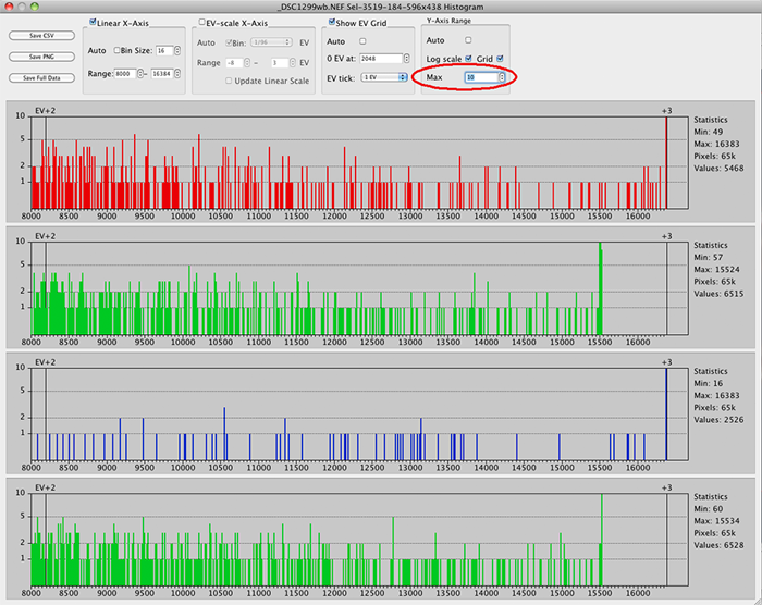
Figure 31 Y-axis. Changing Max value

And the only feature that we haven't touched yet is how to save the histogram.

We see at the top left corner of the histogram window that we have three Save options.

Note: If the histogram data is to be processed further in a spreadsheet or by some other means Save CSV and Save Full Data options offer csv/txt format. To capture just “the look” of the histogram and prepare a screenshot for publishing Save PNG can be used.

1) Save histogram as .csv or .txt:

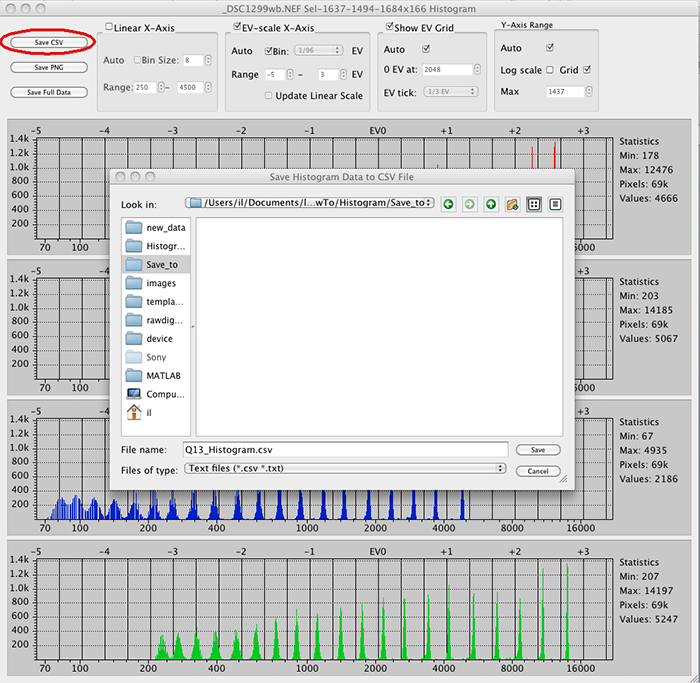
Figure 32.

2) Save it as a .png file:

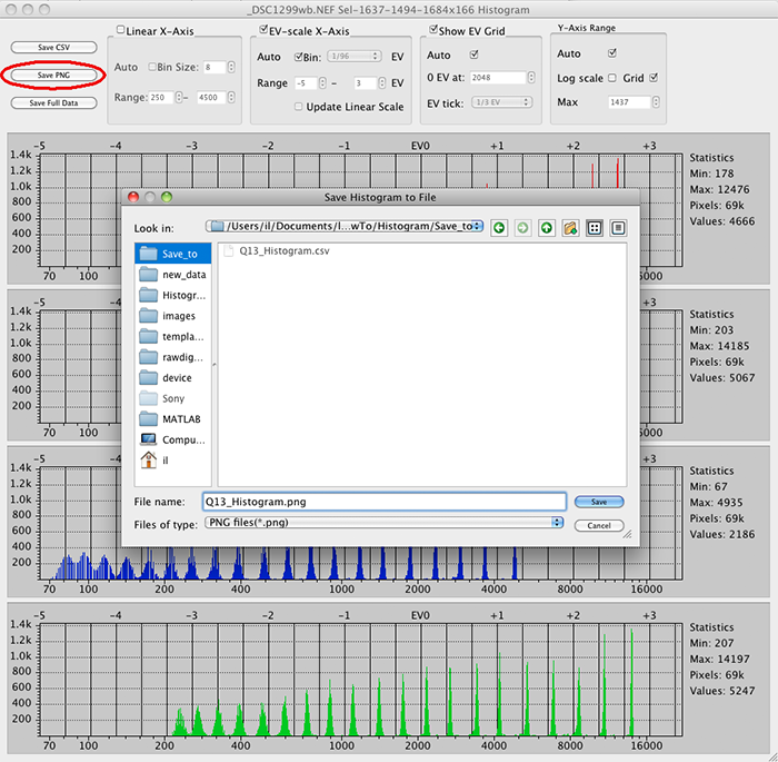
Figure 33.

3) Save full raw data – in .csv format:

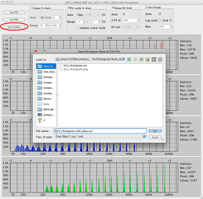
Figure 34.

RAW files used in this text

• Q13_RGBG16.dng - Q13 simulation, use exiftool to extract reference values:
  
  exiftool -usercomment -b Q13_RGBG16.dng >Q13.csv
• _DSC1299.NEF - real Q13 shot

The Unique Essential Workflow Tool

for Every RAW Shooter

FastRawViewer is a must have; it's all you need for extremely fast and reliable culling, direct presentation, as well as for speeding up of the conversion stage of any amounts of any RAW images of every format.

Now with Grid Mode View, Select/Deselect and Multiple Files operations, Screen Sharpening, Highlight Inspection and more.