Lossy compression of raw data is currently the only option available in Sony cameras of series NEX, SLT, RX, ILCE, ILCA, and the recent DSLR-A. The first part of this article is showing how to detect artifacts caused by this compression. We will be discussing the technical details of this compression in the second part of this article.

In the vast majority of cases, the compression artifacts are imperceptible unless the heavy-handed contrast boost is introduced. There are, however, exceptions. With some unlucky stars in alignment, the artifacts can become plainly visible, even without much image processing.  All that is necessary for the artifacts to threaten the quality of the final image is a combination of high local contrast and a flat featureless background.

Lets have a look at the example provided by Matti Koski, it is the same example that was published by Lloyd Chambers in his blog. Upd.: Many thanks to Mr. Koski who now gave us his permission to link to the original raw file _DSC0035-startrails.ARW

The artifacts in the form of a horizontal color fringe on both sides of one of the star trails are very visible even if all of the sliders are set to zero, except the exposure slider:

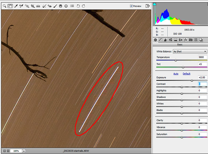
Figure 1. Star Trails. Shot opened in Adobe Camera Raw

This problem is even more visible in RawDigger, because for display purposes, RawDigger employs a variant of Auto Levels, when the tones of the image are stretched to occupy the whole tonal range:

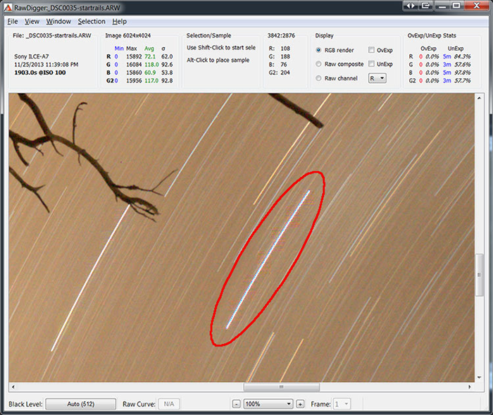
Figure 2

What we have here is a clear case of posterization, which is the lack of continuous gradation of tone, or, in other words, color quantization. It is caused by a sort of rounding error specific to the compression scheme Sony are using for there cRAW format. This error occurs when the step between values in the 16-byte block being too crude (a detailed explanation of the mechanism is in the «Inside SONY cRAW format» part of this article, below). As a result of this rounding error, the artifacts are visible even without moving the contrast slider to the right.

To detect the problematic areas in images captured in Sony cRAW format, RawDigger, starting with the version 1.0.5, offers a special unpacking and display mode, which can be switched on with:

Preferences – Data Processing – Sony ARW2 processing mode – Processing mode: Delta step relative to value

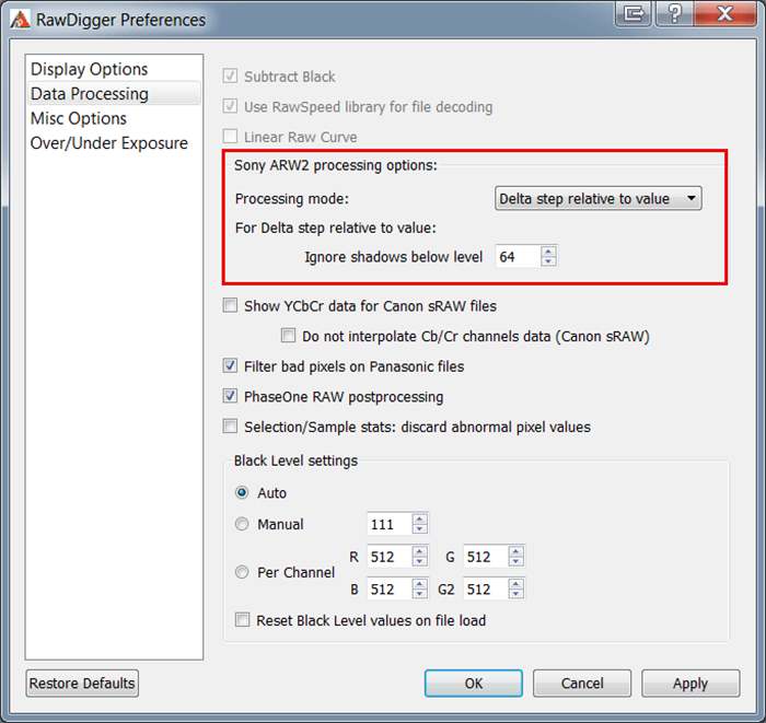
Figure 3

In this mode, instead of a regular procedure of data unpacking, we calculate the degree of posterization, that is, the ratio of the minimum variation of data (data step) in the 16-pixel block to the value of the pixel. This ratio is in per mil (1/1000, ‰). Consequently, the ratios of several tens per mil (that is several percent) may be visible if the background is a smooth gradient. Several hundreds per mil (that is several tens of percent) will certainly be visible if the background is smooth and featureless.

Here is the same area of the star trails shot displayed in Delta step relative to value mode:

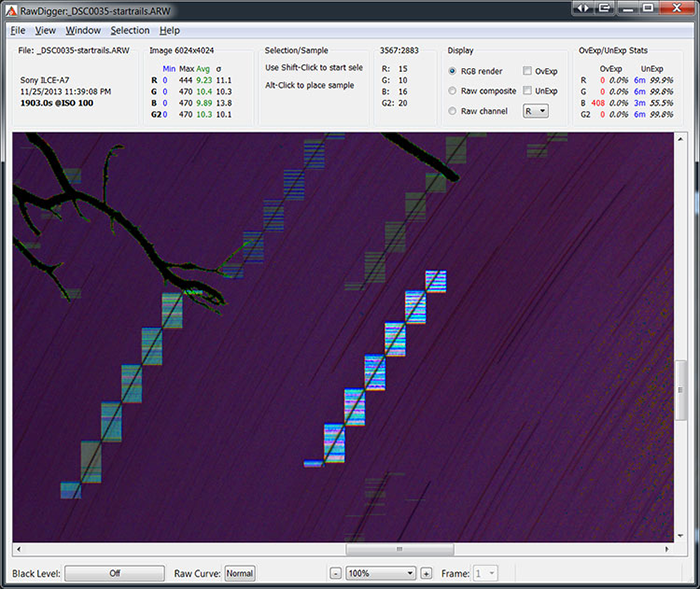
Figure 4

As you can see, the areas containing artifacts can be easily detected. These areas may exhibit posterization on the final image. 

With a little effort we can make this mode even more usable.

Suppose we want to select the areas where the degree of posterization is 10% (100‰). To do so in RawDiggerer Preferences – Over/Under Exposure we set the Manual level all channels in Overexposure Detection group to 100:

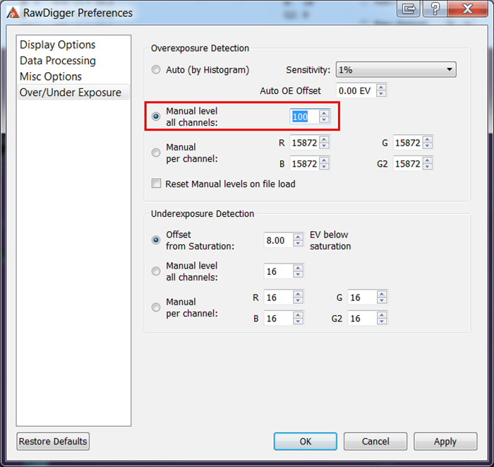
Figure 5

Switching on the indication of Overexposure (check mark in OvExp) we will see a red overlay over the areas where the degree of posterization is higher than 10%:

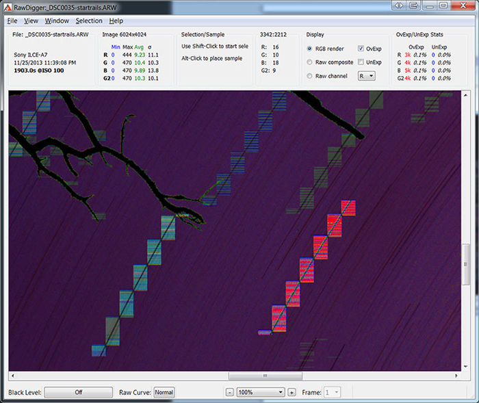
Figure 6

In this mode, the areas of potential posterization are displayed over the whole image. However, on the final image, posterization will be visible only over smooth and featureless backgrounds like sky, sometimes eye whites, and flat shadows. In all other cases, the only effect of this posterization is an error in local color reproduction. There is very little chance that this error will be discernible.

Let’s take a look at the following shot (from Quesabesde's Sony A7R analysis page):

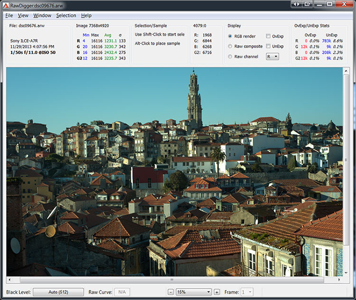
Figure 7

All of the hard contrast edges exhibit some artifacts where one can suspect posterization:

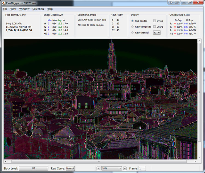
Figure 8

However, on the final image the posterization is visible only on the edge of the tower where the background is a featureless blue sky.

We will use this shot to demonstrate an additional setting, which helps to exclude the lowest tone values (deep shadows) from the posterization map.

Deep shadows always contain hidden, but substantial posterization because only a few levels are present there. Even if the encoding is lossless, the minimal step in the shadows of a cRAW file is equal to 2. This means that if the level is 64, the degree of posterization is more than 30‰ (2/64 = 3.125%).

In order to keep the display of the image cleaner, you can use the Ignore shadows below level NN setting. This setting is active only together with Sony ARW2 Processing – Delta Step relative to value.

If this setting is turned off (that is, the value in the field is set to zero), the scene will show additional posterization in the shadows on the foreground:

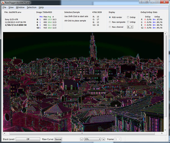
Figure 9

Inside SONY cRAW format

Sony cRAW files are packed and unpacked as following:

1. Data coming from the sensor is biased by the black level (for example, for Sony A7r camera black level is 512 and this value is added to all the data) and is compressed through the tone curve equivalent to the one below; the compressed result contains 11-bit values.

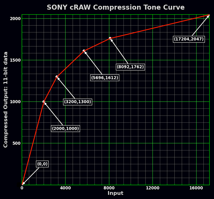
Figure 10

2. Each data row (a row has the height of 1 pixel) is split into 32-pixel chunks, each chunk containing interleaved pixels from 2 color channels. For odd rows a chunk contains 16 R-pixels and 16 G-pixels (RGRGRG…), for even rows it contains 16 G-pixels and 16 B-pixels (GBGBGB…)

3. The structure of each 16-pixel block is:

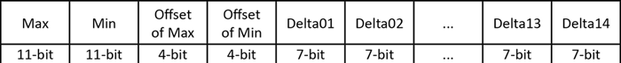
Figure 11

Here, Max is the maximum pixel value in the block, Min is the minimum value in the block, Offsets are the positions of pixels with Max and Min values relative to the block start

Deltas are calculated as:

DataSpan = Max – Min

Step = 2^{rounding(log2(DataSpan/128))}

Delta = (PixelValue – Min) / Step (see more on this below)

The length of the block is 2*11+2*4+14*7=128 bits, or 16 bytes. Thus the raw data compressed per cRAW scheme effectively uses 1 byte per pixel; but the total ARW2 file size is slightly larger as it contains not only cRAW data, but also metadata and JPEG preview.

The larger the data span in a 16-pixel block is, the larger the step is, which is multiplied by the delta value to restore the pixel value, and consequently the larger the data step is. For a data span of less than or equal to 128, the factor is 1, and no rounding error is introduced while reversing the delta encoding. For a larger span, the scheme does introduce the rounding error, which may lead to posterization. In other words, if the chunk of 32 pixels spans across an area that contains a large variation in brightness, the data in the block is not exact, but is only an approximation.

4. During the raw conversion, first, the delta encoding is reversed, next, the linearization tone curve (contained in the metadata of Sony ARW2 files) is applied to decompress the data, and finally the black level (also taken from metadata) is subtracted from the result.

After black level subtraction Sony cRAW linearization tone curve is effectively this:

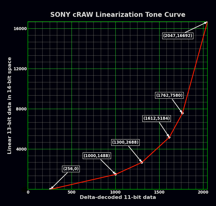
Figure 12. Sony cRAW tone curve with black level being subtracted

Or, in a form of a table:

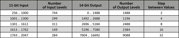
Figure 13

Consider the star trails shot once again:

Figure 14

Inspecting the green channel, we can see that the RAW values in the proximity of the track (black level is subtracted) are:

• The star trail proper has pixel values that reach as high as 4080
• The sky around the trail is a smooth featureless background, and the pixel values close to the trail range from 80 to 200.

Applying compression tone curve to this data:

• The maximum value is 1474 (compression applied to 4080)
• The minimum value is 296 (compression applied to 80)

Data span = (max – min) = (1474 – 296) = 1178.

In order to code values up to 1178 in 7 bits we need to set the step to 16: 2^ceiling(log₂^(1178/128)) = 16.

In other words, for a data span of 1178 the nearest larger number that is an exact power of 2 is 2048 = 2¹¹. Dividing 2048 by 128, we have the step of 16.

The delta values during the decompression are multiplied by this step and further decompressed through the curve which you can dump using RawDigger. In our example, after performing decompression through the tone curve the step of 16 becomes 32, that is ≈14-30% of the values characteristic to the background. Naturally with such a crude step posterization becomes plainly visible.

Other Modes under ARW2 Data Processing

Since we have already discussed cRAW/ARW2 format, it is easier to understand the other options under Sony ARW2 Data processing:

• Standard processing – regular unpacking of RAW data
• Only base pixels – those pixels where the precise 11-bit values are coded (min and max in the block) are unpacked, while for all other pixels (Delta pixels) are set to zero.
• Only delta pixels – Delta pixels are unpacked, and adding the minimum value restores their values, after that the base pixels are set to zero.
• Delta pixels relative to zero – same as previous setting but minimum values are not added to Delta pixels.
• This mode is also, like the one below, useful for determining the area where the posterization may occur. However now we have added more tale-telling mode, that is the one below.

• Delta step relative to value – this mode was used throughout the whole article.

This article in PDF format: RawDigger_Detecting_Posterization_in_Sony_Camera.pdf

The Unique Essential Workflow Tool

for Every RAW Shooter

FastRawViewer is a must have; it's all you need for extremely fast and reliable culling, direct presentation, as well as for speeding up of the conversion stage of any amounts of any RAW images of every format.

Now with Grid Mode View, Select/Deselect and Multiple Files operations, Screen Sharpening, Highlight Inspection and more.