We often hear “my camera has not enough dynamic range”, or “the numbers on that and that review site suggest that many stops of the dynamic range, but I do not see it, my highlights are blown out, my shadows are noisy and blotchy”. Part of the problem is in how one sets the exposure. To set the exposure correctly it is good to know how the in-camera light meter works, and how it is calibrated. So, what is exposure meter calibration and why is it important?

Understanding of the exposure meter calibration determines the outcome of the exposure. The in-camera exposure meter is strictly a reflected-light meter, meaning that it can only register the light that reflects off of a given object back into the meter through the camera lens. Moreover, it will cause whatever is measured to be rendered as the medium tone (also called midtone, and often referred to as 18%). What does this mean? Well, let’s take a closer look.

On the opposite sides of the brightness scale are soot-black and titanium white. Titanium white reflects slightly more than 97% of light, while soot-black reflects only about 2% or less. Directly in between them is a sort of “middle” gray. However, unlike what you might think, this gray does not reflect 50% of light. Instead, it reflects about 18%. The light meter has no way of knowing if it is pointed to white, black, gray, or something else. It tends to consider any scene to be of the average of 18% reflectivity, meaning your camera believes that the whole scene or an object under your light meter reflects those proverbial 18% of light.

Incidentally, those 18% are 2.47 stops (EV) below the overexposure indication in the camera:

log₂(100/18) = 2.47

From this we can deduce that the calibration point for out-of-camera JPEGs is close to 2.5 stops below the overexposure.

This is true (and useful) if you are allowing the camera to process your shots into out-of-camera JPEGs. However if you are shooting in RAW and willing to maximize the useful dynamic range the camera can capture you may want to have a little more flexibility. This is where it becomes necessary to determine the “RAW” calibration point of the light meter, because quite often it is very different from 18%. Moreover, for the same camera it may vary with the camera ISO setting. You can benefit from knowing where this point is for the cameras and camera settings that you are using.

Suppose you are going to take a photo of a high contrast scene (or, in other words, high dynamic range scene), like a downhill skier. This is not a scenario that is easy to work with – it’s heavily backlit (leading to contre-jour, or silhouette, effect, not what you probably want here), with the background being either the sky or the snow (or even both), and the main subject of our scene is not even in it while we are getting ready for the shot. What are our options? Well, we can set the exposure based solely on the snow, but that option should be immediately discarded, because should we go by this route, the snow will be rendered middle gray, and the skier will become pitch-black (by the way, this is often the outcome of leaving the exposure totally to the camera judgment). This is where knowing your camera’s calibration point comes in extremely handy.

For example, in the course of the experiment below you have determined that the exposure meter calibration point in RAW is at 11%, that is there are log₂(100/11) = 3.18 stops between the exposure meter readings and overexposure. Now we can tune the exposure settings so that the snow becomes brighter, whiter, and saving the skier – just by adding the exposure compensation of 3 EV to the exposure meter readings from the snow, and we will still maintain snow’s texture, not turning it into a blind featureless area; while lifting the shadows (and the skier) as high as possible.

To establish the point to which the camera’s exposure meter is calibrated, one can use the following procedure:

1. We prepare a shoot as the following:
   • Choose a featureless matte unicolored surface (such as a grey card, or a wall), relatively evenly lit;
   • Set the camera on the tripod
   • Stop the lens down one or two f-stops (say, if your fully opened lens has an aperture of f/4, stop it down to f/5.6 or f/8)
   • Defocus the lens until the texture of the surface looks blurred, make a trial shot and examine it to confirm
2. We take the first shot of the series with an exposure set exactly to the readings of the in-camera exposure meter activated in the spot-metering mode
3. Then, we take a series of shots, decreasing the shutter speed (and thus increasing the exposure) with every shot (for instance, by 0.3 or 0.5EV) – till +5 stops of overexposure compared to the meter readings
   

   We used the Olympus E-P2 camera, ISO 200, increasing the exposure each time by 1/3 EV.

4. While shooting we note the filename of the first shot on which the in-camera overexposure diagnostics kicks in for the center portion of the shot, and we record the exposure parameters for that shot (or find them out through EXIF later, in RawDigger) – and continue shooting the series until we reach +5 EV over the exposure meter.
5. When finished shooting we open RawDigger and check that in Preferences, RawDigger is set thusly:
   
   

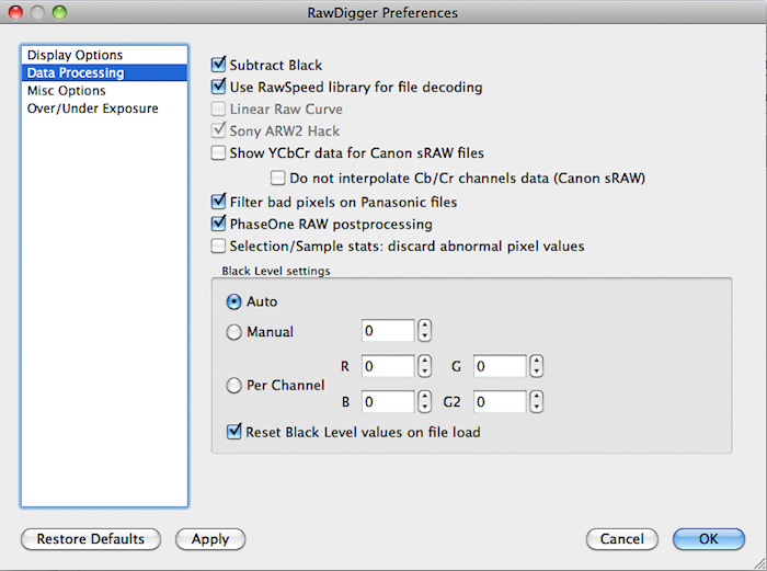
   Figure 1.

   While the Auto mode is active for the Black Level settings, the numbers for the black level in the Manual and Per Channel fields do not matter.

6. We open the first shot of our series, the one that was taken by the exposure meter, with the help of RawDigger.
7. We set the overexposure warning (the Ov.Exp checkmark in the Display section, see Figure 2)
8. With the help of Shift-Click’n’Drag, we choose a small zone, approximately at the center of the shot
   
   (a good size is between 200x200 and 400x400 pixels, the position of the upper left corner of the selected zone and the dimensions of the selection are displayed in the header of third column to the left on the information bar).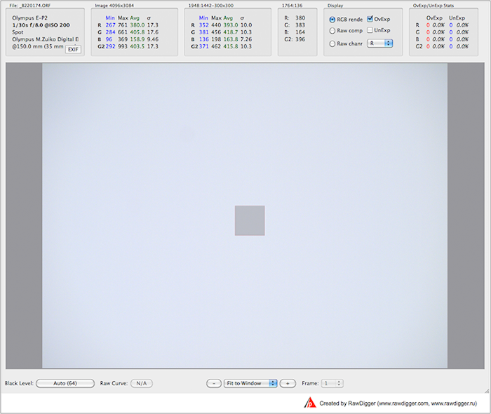
   

   Figure 2.

   Note:
   
   another method of setting the zone – in the “Selection” menu, choose “Set Selection by Numbers” option, and in the pop-up, set the position for the top left corner of the square, as well as its height and width. Determining the position of the zone is easy, using the information about the size of the image (second column to the left of the information bar, titled “Image: Width x Height”). In our case, it’s 4096x3084. Divide each by 2, subtract half of the desired zone size, and enter the coordinates and the size.

9. The section third from the left in the upper information bar contains the statistics for the selected zone – the position of the top left corner, size and, what is most important for our study, the minimum, maximum, average, and standard deviation (σ) values for the R, G and B channels.
10. Let’s record then average value and standard deviation σ for the green channel G (in our case, 418.7 and 10.3, respectively) for the selected zone
11. Now, we determine practical channel maximum value by adding 2*σ to the average. In our case, the maximum is now 418.7 + 2*10.3 = 439.3 – that includes 95% of the pixel values to the right of the average and is more than enough for any practical purpose.
12. Then, we open shots in the series in order, until we reach the shot in which the RawDigger indicator shows some overexposed pixels in the selected zone (reddish dots on the image are that indicator):
    
    

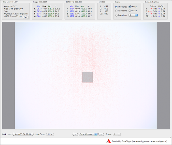
    Figure 3.

    When opening sequential shots, it is unnecessary to select the zone again, because it saves.

    Opening the next shot is easy to do in the File/Next File menu, or with the help of the corresponding shortcut.

    If opened in automatic mode, the histogram of the selected zone looks like this:

    

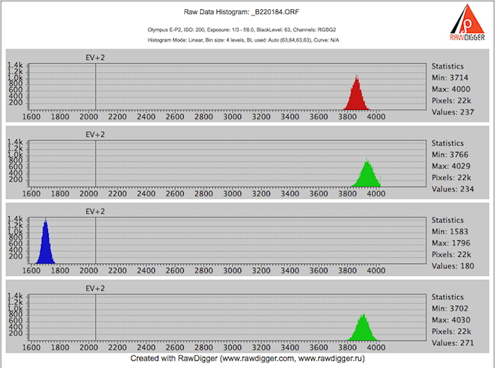
    Figure 4.

    A sharp spike is clearly visible on the right edge of the G channel histogram, and the maximum value corresponding to this spike is in our case 4029 (you can see it to the right of the G channel histogram).

13. So, from this shot we determined the maximum value for the green channel G.

    This value corresponds to the point where the sensor is saturated in the G channel. The spike to the right also often referred to as “histogram hits the wall”, is the tell-tale sign for channel saturation.

14. To determine how many EV (exposure stops) are between the shot exposed by the exposure meter and the shot where we determined the actual overexposure in the raw data, let’s divide the maximum value (the one we just found) by the mean value of the green channel from the first shot in the series (the one which was taken exactly as the exposure meter advised), calculate the logarithm base 2 of the result, and round it down.

    In our case, this value is log₂(4029/418.7) = 3.27. It is easy to see that this encompasses a little more than 3 ¼ EV. For practical applications, we round it to 3 EV (and this way we also have some room for the raw converter’s job – more than ¼ of a stop).

15. To guarantee fully textured highlights let’s divide the maximum (as per above) by the value we obtained by adding 2*σ to the green channel average from the first shot of the series (once again, it was the shot which was exposed according to the exposure meter), calculate the logarithm base 2 of the result and round it down.

    In our case, this is log₂(4029/ 439.3) = 3.2. Round this to 3 EV. So we see that estimating the same 3 EV difference between the readings of the exposure meter and the detailed highlights is safe.

16. We can set the question in another manner – what percentage of gray the exposure by the meter renders?

    To determine this, we divide the maximum green channel value from the overexposed shot by the average in the green channel from the first shot in the series, and multiply by 100%

    In our case, we get 418.7/4029*100% = 10.39%. In relation to the standard 18%, this creates an underexposure of the midtone by log₂(18/10.39) = 0.8 EV. By default, the compensation for the underexposed midtones happens with the help of the tone curve during raw conversion process; but now it is you having the control, and you may choose to expose hotter, thus having less noise and more resolution in shadows.

17. The headroom in the highlights is the difference in exposure between the shot for which the in-camera diagnostics shows overexposure, and the shot in which there is a visible overexposure in the raw data.

    In our case, the camera diagnostics marks as completely overexposed the shot that is taken with a shutter speed of ¼ of a second.

    This is how this shot looks on the camera screen:

    

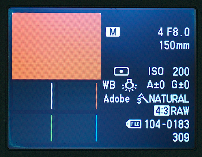
    Figure 5.

    And this is what the histogram of the selected zone (frame center) shows for the same shot in RawDigger:

    

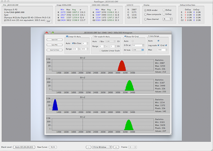
    Figure 6.

    Notice, that no saturation in highlights in fact happens.

    And only for the shot, taken with a shutter speed of 0.4 sec (2 steps of 1/3 EV each higher than the shot which was “trashed” by the camera), RawDigger shows a considerable overexposure:

    

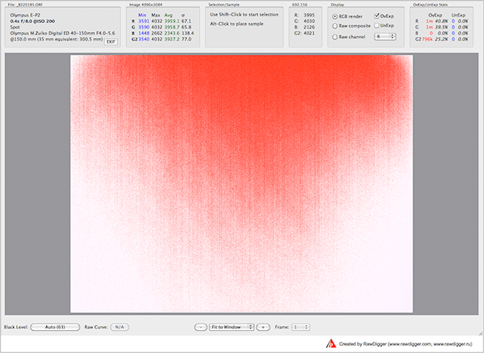
    Figure 7.

    It is easy to see, that the difference in exposure between these two shots is log₂(0.4/0.25) = 2/3 EV. In other words, the exposure for the shot, which was “trashed” by the camera, is 2/3 EV lower than the exposure for the shot in which we can see saturated raw data (saturation encompasses around 40% of pixels in the R and G channels).

    The result is this: 2/3 EV of positive exposure compensation over the readings of the in-camera exposure meter is the practical limit for the measurements in spot mode for the camera that we used.

    It is important to note that the result for the headroom depends not only on the camera model, but it also could be changed with the color space settings, sharpening, contrast, highlight protection, and other camera settings. Sometimes the headroom in highlights and the calibration could be changed with the firmware update. The dirt getting into the camera and obstructing the light meter may skew the exposure readings and can be easily diagnosed with the above procedure. Multi-pattern, evaluative, matrix metering modes may overcome metering calibration completely. Calibration point is most useful when well-defined metering modes, such as spot or center-weighted average metering, are in use.

    It is good to repeat this simple procedure once in a while to ensure the camera stays within the initial factory calibration.

    Similar procedure can be used to verify the progression of the aperture for each lens, and the progression of the shutter speeds. The errors in the progressions due to malfunctions or going out of calibration are easily recognizable by the graphs of average values plotted in a spreadsheet.
    
    But that is for our next story.

The Unique Essential Workflow Tool

for Every RAW Shooter

FastRawViewer is a must have; it's all you need for extremely fast and reliable culling, direct presentation, as well as for speeding up of the conversion stage of any amounts of any RAW images of every format.

Now with Grid Mode View, Select/Deselect and Multiple Files operations, Screen Sharpening, Highlight Inspection and more.